

12
Sverdrup Theory
even though the stress is. The geostrophic region, in which the turbulent
stresses vanish, is also set in motion. How this happens is an important part of
the story that we spend much time in developing below, but at this stage it is
illuminating and also useful for our later discussion to understand at least how
the geostrophic region considered as a whole is set in motion, even though the
turbulent stresses vanish there (at least to lowest order).
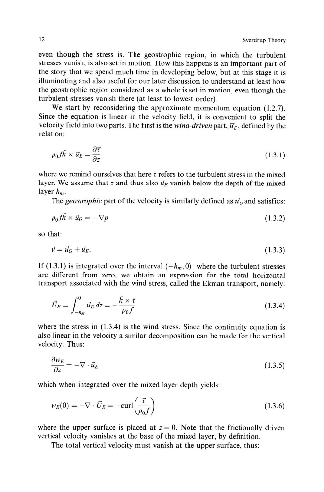
We start by reconsidering the approximate momentum equation (1.2.7).
Since the equation is linear in the velocity field, it is convenient to split the
velocity field into two parts. The first is the wind-driven part, uE, defined by the
relation:
A
8f
Pofk X U£ = az
(1.3.1)
where we remind ourselves that here r refers to the turbulent stress in the mixed
layer. We assume that rand thus also U£ vanish below the depth of the mixed
layer hm.
The geostrophic part of the velocity is similarly defined as ita and satisfies:
Poft x iic = -'\lp
( 1.3.2)
so that:
ii = iic + U£.
( 1.3.3)
If (1.3.1) is integrated over the interval ( -hm, 0) where the turbulent stresses
are different from zero, we obtain an expression for the total horizontal
transport associated with the wind stress, called the Ekman transport, namely:
~
lO
k X T
UE =
U£dZ = - - -
-hM
Poi
(1.3.4)
where the stress in (1.3.4) is the wind stress. Since the continuity equation is
also linear in the velocity a similar decomposition can be made for the vertical
velocity. Thus:
which when integrated over the mixed layer depth yields:
wE(O) = -'\1 · th =-curl(_!_) Poi
(1.3.5)
(1.3.6)
where the upper surface is placed at z = 0. Note that the frictionally driven
vertical velocity vanishes at the base of the mixed layer, by definition.
The total vertical velocity must vanish at the upper surface, thus:
Sverdrup Theory
even though the stress is. The geostrophic region, in which the turbulent
stresses vanish, is also set in motion. How this happens is an important part of
the story that we spend much time in developing below, but at this stage it is
illuminating and also useful for our later discussion to understand at least how
the geostrophic region considered as a whole is set in motion, even though the
turbulent stresses vanish there (at least to lowest order).
We start by reconsidering the approximate momentum equation (1.2.7).
Since the equation is linear in the velocity field, it is convenient to split the
velocity field into two parts. The first is the wind-driven part, uE, defined by the
relation:
A
8f
Pofk X U£ = az
(1.3.1)
where we remind ourselves that here r refers to the turbulent stress in the mixed
layer. We assume that rand thus also U£ vanish below the depth of the mixed
layer hm.
The geostrophic part of the velocity is similarly defined as ita and satisfies:
Poft x iic = -'\lp
( 1.3.2)
so that:
ii = iic + U£.
( 1.3.3)
If (1.3.1) is integrated over the interval ( -hm, 0) where the turbulent stresses
are different from zero, we obtain an expression for the total horizontal
transport associated with the wind stress, called the Ekman transport, namely:
~
lO
k X T
UE =
U£dZ = - - -
-hM
Poi
(1.3.4)
where the stress in (1.3.4) is the wind stress. Since the continuity equation is
also linear in the velocity a similar decomposition can be made for the vertical
velocity. Thus:
which when integrated over the mixed layer depth yields:
wE(O) = -'\1 · th =-curl(_!_) Poi
(1.3.5)
(1.3.6)
where the upper surface is placed at z = 0. Note that the frictionally driven
vertical velocity vanishes at the base of the mixed layer, by definition.
The total vertical velocity must vanish at the upper surface, thus: