

212
Theory of the Ventilated Thermocline
Zn+i
(4.7.17)
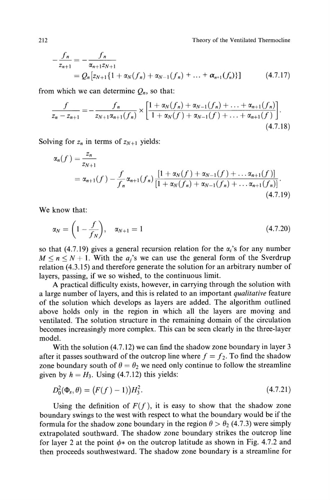
from which we can determine Qn, so that:
J
fn
[1 + (J.N(fn) + (J.N-i (/n) + · · · + (J.n+i (/n)]
Zn-Zn+l =-ZN+l(J.n+l(fn)X 1+(J.N(f)+(J.N-i(f)+ ... +(J.n+i(f) .
(4.7.18)
Solving for Zn in terms of ZN+i yields:
We know that:
(J.N = ( 1 - £), (J.N+i = 1
(4.7.20)
so that (4.7.19) gives a general recursion relation for the (J.;'s for any number
M :::; n :::; N + 1. With the a/s we can use the general form of the Sverdrup
relation (4.3.15) and therefore generate the solution for an arbitrary number of
layers, passing, if we so wished, to the continuous limit.
A practical difficulty exists, however, in carrying through the solution with
a large number of layers, and this is related to an important qualitative feature
of the solution which develops as layers are added. The algorithm outlined
above holds only in the region in which all the layers are moving and
ventilated. The solution structure in the remaining domain of the circulation
becomes increasingly more complex. This can be seen clearly in the three-layer
model.
With the solution (4.7.12) we can find the shadow zone boundary in layer 3
after it passes southward of the outcrop line where f = h· To find the shadow
zone boundary south of 8 = 82 we need only continue to follow the streamline
given by h = H3. Using ( 4. 7 .12) this yields:
(4.7.21)
Using the definition of F(f ), it is easy to show that the shadow zone
boundary swings to the west with respect to what the boundary would be if the
formula for the shadow zone boundary in the region 8 > 82 (4.7.3) were simply
extrapolated southward. The shadow zone boundary strikes the outcrop line
for layer 2 at the point¢* on the outcrop latitude as shown in Fig. 4.7.2 and
then proceeds southwestward. The shadow zone boundary is a streamline for
Theory of the Ventilated Thermocline
Zn+i
(4.7.17)
from which we can determine Qn, so that:
J
fn
[1 + (J.N(fn) + (J.N-i (/n) + · · · + (J.n+i (/n)]
Zn-Zn+l =-ZN+l(J.n+l(fn)X 1+(J.N(f)+(J.N-i(f)+ ... +(J.n+i(f) .
(4.7.18)
Solving for Zn in terms of ZN+i yields:
We know that:
(J.N = ( 1 - £), (J.N+i = 1
(4.7.20)
so that (4.7.19) gives a general recursion relation for the (J.;'s for any number
M :::; n :::; N + 1. With the a/s we can use the general form of the Sverdrup
relation (4.3.15) and therefore generate the solution for an arbitrary number of
layers, passing, if we so wished, to the continuous limit.
A practical difficulty exists, however, in carrying through the solution with
a large number of layers, and this is related to an important qualitative feature
of the solution which develops as layers are added. The algorithm outlined
above holds only in the region in which all the layers are moving and
ventilated. The solution structure in the remaining domain of the circulation
becomes increasingly more complex. This can be seen clearly in the three-layer
model.
With the solution (4.7.12) we can find the shadow zone boundary in layer 3
after it passes southward of the outcrop line where f = h· To find the shadow
zone boundary south of 8 = 82 we need only continue to follow the streamline
given by h = H3. Using ( 4. 7 .12) this yields:
(4.7.21)
Using the definition of F(f ), it is easy to show that the shadow zone
boundary swings to the west with respect to what the boundary would be if the
formula for the shadow zone boundary in the region 8 > 82 (4.7.3) were simply
extrapolated southward. The shadow zone boundary strikes the outcrop line
for layer 2 at the point¢* on the outcrop latitude as shown in Fig. 4.7.2 and
then proceeds southwestward. The shadow zone boundary is a streamline for