

116
Vertical Structure: Baroclinic Quasi-Geostrophic Models
the bottom topography, either because we (unrealistically) assume in our
model that the bottom is fiat, or that our model is a two-layer model over a
resting abyss that shelters the layers from the effect of the topography (as well
as bottom friction, of course). With these assumptions the equation for the
vertical average of the interior motion once again becomes the Sverdrup
balance:
(3.5.6)
where:
(3.5. 7)
and H = H1 +H2.
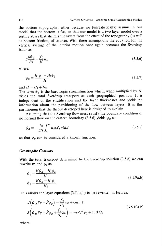
The term t/Js is the barotropic streamfunction which, when multiplied by H,
yields the total Sverdrup transport at each geographical position. It is
independent of the stratification and the layer thicknesses and yields no
information about the partitioning of the flow between layers. It is this
partitioning that the theory developed here is designed to explain.
Assuming that the Sverdrup flow must satisfy the boundary condition of
no normal flow on the eastern boundary (3.5.6) yields t/Js as:
t/Js = - f; 1xe wE(x', y)dx'
(3.5.8)
so that t/1 B can be considered a known function.
Geostrophic Contours
With the total transport determined by the Sverdrup solution (3.5.8) we can
rewrite lf/1 and lf/2 as:
t/11 = Ht/Js - H2t/J2
H1
t/12 = Ht/Js- Hlt/11.
H2
(3.5.9a,b)
This allows the layer equations (3.5.4a,b) to be rewritten in turn as:
(3.5.10a,b)
where:
Vertical Structure: Baroclinic Quasi-Geostrophic Models
the bottom topography, either because we (unrealistically) assume in our
model that the bottom is fiat, or that our model is a two-layer model over a
resting abyss that shelters the layers from the effect of the topography (as well
as bottom friction, of course). With these assumptions the equation for the
vertical average of the interior motion once again becomes the Sverdrup
balance:
(3.5.6)
where:
(3.5. 7)
and H = H1 +H2.
The term t/Js is the barotropic streamfunction which, when multiplied by H,
yields the total Sverdrup transport at each geographical position. It is
independent of the stratification and the layer thicknesses and yields no
information about the partitioning of the flow between layers. It is this
partitioning that the theory developed here is designed to explain.
Assuming that the Sverdrup flow must satisfy the boundary condition of
no normal flow on the eastern boundary (3.5.6) yields t/Js as:
t/Js = - f; 1xe wE(x', y)dx'
(3.5.8)
so that t/1 B can be considered a known function.
Geostrophic Contours
With the total transport determined by the Sverdrup solution (3.5.8) we can
rewrite lf/1 and lf/2 as:
t/11 = Ht/Js - H2t/J2
H1
t/12 = Ht/Js- Hlt/11.
H2
(3.5.9a,b)
This allows the layer equations (3.5.4a,b) to be rewritten in turn as:
(3.5.10a,b)
where: