

The Quasi-Geostrophic Model
103
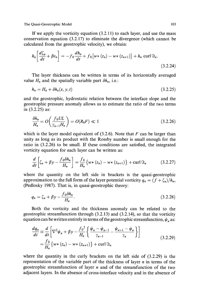
If we apply the vorticity equation (3.2.11) to each layer, and use the mass
conservation equation (3.2.17) to eliminate the divergence (which cannot be
calculated from the geostrophic velocity), we obtain:
(3.2.24)
The layer thickness can be written in terms of its horizontally averaged
value Hn and the spatially variable part bhn, i.e.:
(3.2.25)
and the geostrophic, hydrostatic relation between the interface slope and the
geostrophic pressure anomaly allows us to estimate the ratio of the two terms
in (3.2.25) as:
bhn = o( foUL ) = O(RoF) « l
Hn
Yn-!Hn
(3.2.26)
which is the layer model equivalent of (3.2.6). Note that F can be larger than
unity as long as its product with the Rossby number is small enough for the
ratio in (3.2.26) to be small. If these conditions are satisfied, the integrated
vorticity equation for each layer can be written as:
(3.2.27)
where the quantity on the left side in brackets is the quasi-geostrophic
approximation to the full form of the layer potential vorticity qn = (! + (n)/hn,
(Pedlosky 1987). That is, in quasi-geostrophic theory:
fobhn
qn = (n + f3y- -----n- ·
n
(3.2.28)
Both the vorticity and the thickness anomaly can be related to the
geostrophic streamfunction through (3.2.13) and (3.2.14), so that the vorticity
equation can be written entirely in terms of the geostrophic streamfunction, tjJ n as:
(3.2.29)
where the quantity in the curly brackets on the left side of (3.2.29) is the
representation of the variable part of the thickness of layer n in terms of the
geostrophic streamfunction of layer n and of the streamfunction of the two
adjacent layers. In the absence of cross-interface velocity and in the absence of
103
If we apply the vorticity equation (3.2.11) to each layer, and use the mass
conservation equation (3.2.17) to eliminate the divergence (which cannot be
calculated from the geostrophic velocity), we obtain:
(3.2.24)
The layer thickness can be written in terms of its horizontally averaged
value Hn and the spatially variable part bhn, i.e.:
(3.2.25)
and the geostrophic, hydrostatic relation between the interface slope and the
geostrophic pressure anomaly allows us to estimate the ratio of the two terms
in (3.2.25) as:
bhn = o( foUL ) = O(RoF) « l
Hn
Yn-!Hn
(3.2.26)
which is the layer model equivalent of (3.2.6). Note that F can be larger than
unity as long as its product with the Rossby number is small enough for the
ratio in (3.2.26) to be small. If these conditions are satisfied, the integrated
vorticity equation for each layer can be written as:
(3.2.27)
where the quantity on the left side in brackets is the quasi-geostrophic
approximation to the full form of the layer potential vorticity qn = (! + (n)/hn,
(Pedlosky 1987). That is, in quasi-geostrophic theory:
fobhn
qn = (n + f3y- -----n- ·
n
(3.2.28)
Both the vorticity and the thickness anomaly can be related to the
geostrophic streamfunction through (3.2.13) and (3.2.14), so that the vorticity
equation can be written entirely in terms of the geostrophic streamfunction, tjJ n as:
(3.2.29)
where the quantity in the curly brackets on the left side of (3.2.29) is the
representation of the variable part of the thickness of layer n in terms of the
geostrophic streamfunction of layer n and of the streamfunction of the two
adjacent layers. In the absence of cross-interface velocity and in the absence of