

Reconstructing and Modelling the Last Glacial Maximum
703
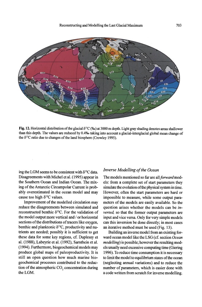
Fig. 12. Horizontal distribution of the glacialS l3 C (%0) at 3000 m depth. Light gray shading denotes areas shallower
than this depth. The values are reduced by 0.4%0 taking into account a glacial-interglacial global mean change of
the Sl3C ratio due to changes of the land biosphere (Crowley 1995).
ing the LGM seems to be consistent with 8 JJ C data.
Disagreements with Michel et al. (1995) appear in
the Southern Ocean and Indian Ocean. The mixing of the Antarctic Circumpolar Current is probably overestimated in the ocean model and may
cause too high 8 JJ C values.
Improvement of the modelled circulation may
reduce the disagreements between simulated and
reconstructed benthic 8 JJ C. For the validation of
the model output more vertical and / or horizontal
sections of the distributions of tracers like oxygen,
benthic and planktonic 813C, productivity and nutrients are needed; possibly it is sufficient to get
these data for some key regions, cf. Duplessy et
al. (1988), Labeyrie et al. (1992), Sarnthein et al.
(1994). Furthermore, biogeochemical models may
produce global maps of paleoproductivity. It is
still an open question how much marine biogeochemical processes contributed to the reduction of the atmospheric CO 2 concentration during
theLGM.
Inverse Modelling of the Ocean
The models mentioned so far are all forward models: from a complete set of start parameters they
simulate the evolution of the physical system in time.
However, often the start parameters are hard or
impossible to measure, while some output parameters of the models are easily available. So the
question arises whether the models can be inverted, so that the former output parameters are
input and vice versa. Only for very simple models
can this inversion be done directly; in most cases
an iterative method must be used (Fig. 13).
Building an inverse model from an existing forward ocean model like the LSG (cf. section Ocean
modelling) is possible; however the resulting models usually need excessive computing time (Giering
1996). To reduce time consumption it is necessary
to limit the model to equilibrium states of the ocean
(neglecting annual variations) and to reduce the
number of parameters, which is easier done with
a code written from scratch for inverse modelling.