

662
Paul eta!'
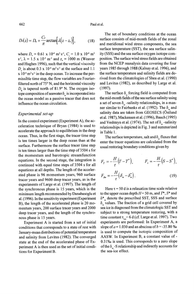
Dv{z) = D. + ~ arctan[ A(Z - z. )],
(18)
where D. = 0.61 X 10. 4 m 2 S-I, C, = 1.0 X 10- 4 m 2
S-I, A = 1.5 X 10- 3 m- I and z. = 1000 m (Weaver
and Hughes 1996), such that the vertical viscosity
Dv is about 0.3 x 10- 4 m 2 S-1 at the surface and 1.1
x 10- 4 m 2 S-1 in the deep ocean. To increase the permissible time step, the flow variables are Fourierfiltered north of7 5 0 N, and the horizontal viscosity
Dh is tapered north of 81.9 0 N. The oxygen isotope composition of seawater Ow is incorporated into
the ocean model as a passive tracer that does not
influence the ocean circulation.
Experimental set-up
In the control experiment (Experiment A), the acceleration technique of Bryan (1984) is used to
accelerate the approach to equilibrium in the deep
ocean. Thus, in the first stage, the tracer time step
is ten times larger in the deep ocean than at the
surface. Furthermore the surface tracer time step
is ten times larger than the time step of3504 s for
the momentum and barotropic stream function
equations. In the second stage, the integration is
continued with equal time steps of3504 s for all
equations at all depths. The length ofthe accelerated phase is 96 momentum years, 960 surface
tracer years and 9600 deep tracer years, as in the
experiments of Large et al. (1997). The length of
the synchronous phase is 15 years, which is the
minimum length recommended by Danabasoglu et
al. (1996). In the sensitivity experiment (Experiment
B), the length of the accelerated phase is 20 momentum years, 200 surface tracer years and 2000
deep tracer years, and the length of the synchronous phase is 15 years.
Experiment A is started from a set of initial
conditions that corresponds to a state of rest with
January-mean distributions of potential temperature
and salinity from Levitus (1982). The converged
state at the end of the accelerated phase of Experiment A is then used as the set of initial conditions for Experiment B.
The set of boundary conditions at the ocean
surface consists of mid-month fields of the zonal
and meridional wind stress components, the sea
surface temperature (SST), the sea surface salinity (SSS) and the sea surface oxygen isotope composition. The surface wind stress fields are obtained
from the NCEP reanalysis data covering the four
years 1985 through 1988 (Kalnay et al. 1996), and
the surface temperature and salinity fields are derived from the climatologies of Shea et al. (1990)
and Levitus (1982), as described by Large et al.
(1997).
The surface Ow forcing field is computed from
the mid-month fields of the sea surface salinity using
a set of seven Ow -salinity relationships, in a manner similar to Fairbanks et al. (1992). The ° and
salinity data are taken from GEOSECS (6stiund
et al. 1987), Mackensen et al. (1996), Bauch (1995)
and Veshteyn et al. (1974). The set of ° -salinity
relationships is depicted in Fig. 3 and su~marized
in Table 1.
The surface temperature, salt and Ow fluxes that
enter the tracer equations are calculated from the
usual restoring boundary conditions given by
F =- H(S_S')
s
,
r
(19)
Here 't = 50 d is a relaxation time scale relative
to the upper ocean depth H = 50 m, and T*, S* and
0* w denote the prescribed SST, SSS and surface
Ow values. The fraction of a grid cell covered by
sea ice is diagnosed from the climatologic SST and
subject to a strong temperature restoring, with a
time constant't i ,,= 6 d (cf. Large et al. 1997). Two
experiments are performed: In Experiment A, a
slope of a = 1.030 and an abscissa of b = -35.80 %0
is used to compute the isotopic composition of
AASW. In Experiment B, a constant value of -
0.3 I %0 is used. This corresponds to a zero slope
ofthe Ow -S relationship and indirectly accounts for
the sea-ice effect.