

216
Wolffetal.
we trained a network with three hidden neurons
using the complete set of core-tops, but only the
35 species which were also counted in the
down core samples. This approach is illustrated and
compared with MAT in Fig. 6.
A general problem ofthe backpropagation training of neural networks is the large computation
expense. We required about a hundred thousand
presentations ofthe reference data before convergence was achieved. The number of necessary
training cycles increases dramatically with the size
of the network. Some computation time could be
saved if the steepest descent strategy which we
use is replaced by a line-search algorithm. Nevertheless, if no special neurocomputer is available, the
expenditure is much larger than for other methods,
such as transfer functions or MAT.
1 . 0 ~------------'
~ 0.8
N
e;
:z 0.6
<;>
'" ' "
.,
.g 0.4
o
o
0>
0.2
0.0'2
3
4
5
number of hidden neurons
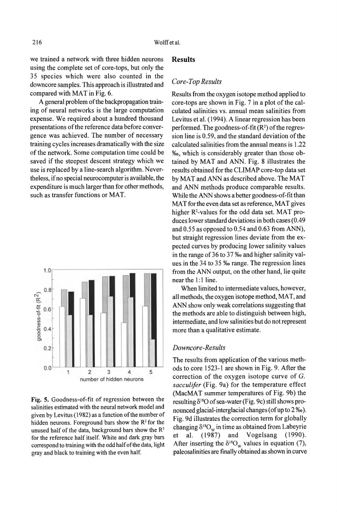
Fig. 5. Goodness-of-fit of regression between the
salinities estimated with the neural network model and
given by Levitus (1982) as a function of the number of
hidden neurons. Foreground bars show the R' for the
unused half of the data, background bars show the R'
for the reference half itself. White and dark gray bars
correspond to training with the odd half of the data, light
gray and black to training with the even half.
Results
Core-Top Results
Results from the oxygen isotope method applied to
core-tops are shown in Fig. 7 in a plot of the calculated salinities vs. annual mean salinities from
Levitus et al. (1994). A linear regression has been
performed. The goodness-of-fit (R') ofthe regression line is 0.59, and the standard deviation ofthe
calculated salinities from the annual means is 1.22
%0, which is considerably greater than those obtained by MAT and ANN. Fig. 8 illustrates the
results obtained for the CLIMAP core-top data set
by MAT and ANN as described above. The MAT
and ANN methods produce comparable results.
While the ANN shows a better goodness-of-fit than
MAT for the even data set as reference, MAT gives
higher R'-values for the odd data set. MAT produces lower standard deviations in both cases (0.49
and 0.55 as opposed to 0.54 and 0.63 from ANN),
but straight regression lines deviate from the expected curves by producing lower salinity values
in the range of36 to 37 %0 and higher salinity values in the 34 to 35 %0 range. The regression lines
from the ANN output, on the other hand, lie quite
near the 1: I line.
When limited to intermediate values, however,
all methods, the oxygen isotope method, MAT, and
ANN show only weak correlations suggesting that
the methods are able to distinguish between high,
intermediate, and low salinities but do not represent
more than a qualitative estimate.
Downcore-Results
The results from application of the various methods to core 1523-1 are shown in Fig. 9. After the
correction of the oxygen isotope curve of G.
sacculifer (Fig. 9a) for the temperature effect
(MacMAT summer temperatures of Fig. 9b) the
resulting 8180 of sea-water (Fig. 9c) still shows pronounced glacial-interglacial changes (of up to 2 %0).
Fig. 9d illustrates the correction term for globally
changing 8 18 0 w in time as obtained from Labeyrie
et al. (1987) and Vogelsang (1990).
After inserting the 8 18 0 W values in equation (7),
paleosalinities are finally obtained as shown in curve
Wolffetal.
we trained a network with three hidden neurons
using the complete set of core-tops, but only the
35 species which were also counted in the
down core samples. This approach is illustrated and
compared with MAT in Fig. 6.
A general problem ofthe backpropagation training of neural networks is the large computation
expense. We required about a hundred thousand
presentations ofthe reference data before convergence was achieved. The number of necessary
training cycles increases dramatically with the size
of the network. Some computation time could be
saved if the steepest descent strategy which we
use is replaced by a line-search algorithm. Nevertheless, if no special neurocomputer is available, the
expenditure is much larger than for other methods,
such as transfer functions or MAT.
1 . 0 ~------------'
~ 0.8
N
e;
:z 0.6
<;>
'" ' "
.,
.g 0.4
o
o
0>
0.2
0.0'2
3
4
5
number of hidden neurons
Fig. 5. Goodness-of-fit of regression between the
salinities estimated with the neural network model and
given by Levitus (1982) as a function of the number of
hidden neurons. Foreground bars show the R' for the
unused half of the data, background bars show the R'
for the reference half itself. White and dark gray bars
correspond to training with the odd half of the data, light
gray and black to training with the even half.
Results
Core-Top Results
Results from the oxygen isotope method applied to
core-tops are shown in Fig. 7 in a plot of the calculated salinities vs. annual mean salinities from
Levitus et al. (1994). A linear regression has been
performed. The goodness-of-fit (R') ofthe regression line is 0.59, and the standard deviation ofthe
calculated salinities from the annual means is 1.22
%0, which is considerably greater than those obtained by MAT and ANN. Fig. 8 illustrates the
results obtained for the CLIMAP core-top data set
by MAT and ANN as described above. The MAT
and ANN methods produce comparable results.
While the ANN shows a better goodness-of-fit than
MAT for the even data set as reference, MAT gives
higher R'-values for the odd data set. MAT produces lower standard deviations in both cases (0.49
and 0.55 as opposed to 0.54 and 0.63 from ANN),
but straight regression lines deviate from the expected curves by producing lower salinity values
in the range of36 to 37 %0 and higher salinity values in the 34 to 35 %0 range. The regression lines
from the ANN output, on the other hand, lie quite
near the 1: I line.
When limited to intermediate values, however,
all methods, the oxygen isotope method, MAT, and
ANN show only weak correlations suggesting that
the methods are able to distinguish between high,
intermediate, and low salinities but do not represent
more than a qualitative estimate.
Downcore-Results
The results from application of the various methods to core 1523-1 are shown in Fig. 9. After the
correction of the oxygen isotope curve of G.
sacculifer (Fig. 9a) for the temperature effect
(MacMAT summer temperatures of Fig. 9b) the
resulting 8180 of sea-water (Fig. 9c) still shows pronounced glacial-interglacial changes (of up to 2 %0).
Fig. 9d illustrates the correction term for globally
changing 8 18 0 w in time as obtained from Labeyrie
et al. (1987) and Vogelsang (1990).
After inserting the 8 18 0 W values in equation (7),
paleosalinities are finally obtained as shown in curve