

On the Reconstruction of Paleosalinities
215
network approach provides a large class of
nonlinear model functions accompanied by a
matching optimization procedure.
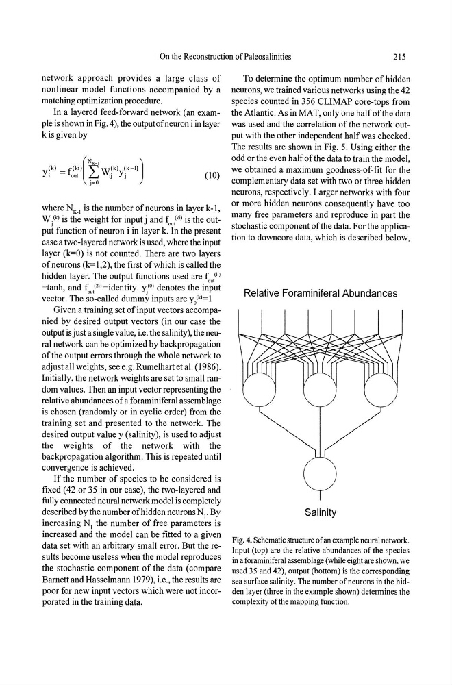
In a layered feed-forward network (an example is shown in Fig. 4), the output of neuron i inlayer
kisgiven by
(
Nk"
J
(k) = f(ki) "W(k) (k-l)
y,
out
L.. IJ YJ
j=O
(10)
where N K • 1 is the number of neurons in layer k-l,
Wi/k) is the weight for inputj and (o?i) is the output function of neuron i in layer k. In the present
case a two-layered network is used, where the input
layer (k=O) is not counted. There are two layers
of neurons (k= 1,2), the first of which is called the
hidden layer. The output functions used are foo?)
=tanh, and foo?i)=identity. yt) denotes the input
vector. The so-called dummy inputs are yo(k)=1
Given a training set of input vectors accompanied by desired output vectors (in our case the
output is just a single value, i.e. the salinity), the neural network can be optimized by backpropagation
ofthe output errors through the whole network to
adjust all weights, see e.g. Rumelhart et al. (1986).
Initially, the network weights are set to small random values. Then an input vector representing the
relative abundances of a foraminiferal assemblage
is chosen (randomly or in cyclic order) from the
training set and presented to the network. The
desired output value y (salinity), is used to adjust
the weights of the network with the
backpropagation algorithm. This is repeated until
convergence is achieved.
If the number of species to be considered is
fixed (42 or 35 in our case), the two-layered and
fully connected neural network model is completely
described by the number of hidden neurons N I' By
increasing NI the number of free parameters is
increased and the model can be fitted to a given
data set with an arbitrary small error. But the results become useless when the model reproduces
the stochastic component of the data (compare
Barnett and Hasselmann 1979), i.e., the results are
poor for new input vectors which were not incorporated in the training data.
To determine the optimum number of hidden
neurons, we trained various networks using the 42
species counted in 356 CLIMAP core-tops from
the Atlantic. As in MAT, only one half of the data
was used and the correlation of the network output with the other independent half was checked.
The results are shown in Fig. 5. Using either the
odd or the even half ofthe data to train the model,
we obtained a maximum goodness-of-fit for the
complementary data set with two or three hidden
neurons, respectively. Larger networks with four
or more hidden neurons consequently have too
many free parameters and reproduce in part the
stochastic component of the data. For the application to downcore data, which is described below,
Relative Foraminiferal Abundances
Salinity
Fig. 4. Schematic structure of an example neural network.
Input (top) are the relative abundances of the species
in a foraminiferal assemblage (while eight are shown, we
used 35 and 42), output (bottom) is the corresponding
sea surface salinity. The number of neurons in the hidden layer (three in the example shown) determines the
complexity ofthe mapping function.
215
network approach provides a large class of
nonlinear model functions accompanied by a
matching optimization procedure.
In a layered feed-forward network (an example is shown in Fig. 4), the output of neuron i inlayer
kisgiven by
(
Nk"
J
(k) = f(ki) "W(k) (k-l)
y,
out
L.. IJ YJ
j=O
(10)
where N K • 1 is the number of neurons in layer k-l,
Wi/k) is the weight for inputj and (o?i) is the output function of neuron i in layer k. In the present
case a two-layered network is used, where the input
layer (k=O) is not counted. There are two layers
of neurons (k= 1,2), the first of which is called the
hidden layer. The output functions used are foo?)
=tanh, and foo?i)=identity. yt) denotes the input
vector. The so-called dummy inputs are yo(k)=1
Given a training set of input vectors accompanied by desired output vectors (in our case the
output is just a single value, i.e. the salinity), the neural network can be optimized by backpropagation
ofthe output errors through the whole network to
adjust all weights, see e.g. Rumelhart et al. (1986).
Initially, the network weights are set to small random values. Then an input vector representing the
relative abundances of a foraminiferal assemblage
is chosen (randomly or in cyclic order) from the
training set and presented to the network. The
desired output value y (salinity), is used to adjust
the weights of the network with the
backpropagation algorithm. This is repeated until
convergence is achieved.
If the number of species to be considered is
fixed (42 or 35 in our case), the two-layered and
fully connected neural network model is completely
described by the number of hidden neurons N I' By
increasing NI the number of free parameters is
increased and the model can be fitted to a given
data set with an arbitrary small error. But the results become useless when the model reproduces
the stochastic component of the data (compare
Barnett and Hasselmann 1979), i.e., the results are
poor for new input vectors which were not incorporated in the training data.
To determine the optimum number of hidden
neurons, we trained various networks using the 42
species counted in 356 CLIMAP core-tops from
the Atlantic. As in MAT, only one half of the data
was used and the correlation of the network output with the other independent half was checked.
The results are shown in Fig. 5. Using either the
odd or the even half ofthe data to train the model,
we obtained a maximum goodness-of-fit for the
complementary data set with two or three hidden
neurons, respectively. Larger networks with four
or more hidden neurons consequently have too
many free parameters and reproduce in part the
stochastic component of the data. For the application to downcore data, which is described below,
Relative Foraminiferal Abundances
Salinity
Fig. 4. Schematic structure of an example neural network.
Input (top) are the relative abundances of the species
in a foraminiferal assemblage (while eight are shown, we
used 35 and 42), output (bottom) is the corresponding
sea surface salinity. The number of neurons in the hidden layer (three in the example shown) determines the
complexity ofthe mapping function.