

214
Wolffetal.
We employed MAT for paleosalinity reconstruction in conjunction with data from core-tops and two
cores ofthe central and south Atlantic. To test the
method, we first applied it to the CLIMAP (1981)
core-top data set (356 samples). The data set was
downloaded from SPECMAP Archive No 1 from
the NOAA ftp server. 42 species counts were included (only abundances of G. ruber total, G.
sacculifer total and G. menardii complex were
excluded to avoid redundancy).
The entire data set was split into two subsets.
This was done by consecutively numbering the
core-tops and then selecting an even-numbered and
an odd-numbered set. The first half was used as a
reference data set, whilst the second was used as
the sample data set, for which annual mean
salinities were computed. The results were compared to the actual sea surface salinities (annual
means) derived from Levitus (1982). In a second
step, the reference and sample data sets were exchanged and computations were performed for the
first half.
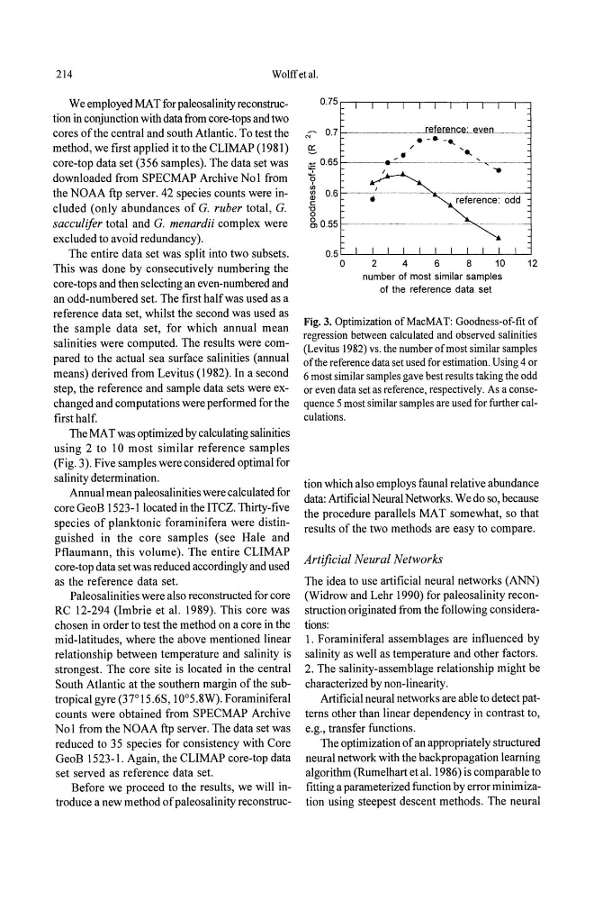
The MAT was optimized by calculating salinities
using 2 to 10 most similar reference samples
(Fig. 3). Five samples were considered optimal for
salinity determination.
Annual mean paleo salinities were calculated for
core GeoB 1523-1 located in the ITCZ. Thirty-five
species of planktonic foraminifera were distinguished in the core samples (see Hale and
Pflaum ann, this volume). The entire CLIMAP
core-top data set was reduced accordingly and used
as the reference data set.
Paleosalinities were also reconstructed for core
RC 12-294 (Imbrie et al. 1989). This core was
chosen in order to test the method on a core in the
mid-latitudes, where the above mentioned linear
relationship between temperature and salinity is
strongest. The core site is located in the central
South Atlantic at the southern margin of the subtropical gyre (37°15.6S, 10 0 5.8W). Foraminiferal
counts were obtained from SPECMAP Archive
No 1 from the NOAA ftp server. The data set was
reduced to 35 species for consistency with Core
GeoB 1523-1. Again, the CLIMAP core-top data
set served as reference data set.
Before we proceed to the results, we will introduce a new method of paleosalinity reconstrucN' 0.7 _____ ~~_~._Je!eJ.e.nc.e;_.e_'l.en ____ _
.. - .. _,
±:: 0.65
~
W
~ 0,6
to
"0
o
g, 0.55
.... ~
...........
---,-'''-,---.--"-,,-,--,, -
--_.- --.-" .... ~
-.
reference: odd
0.5 '---"'----'---'---'----'----''-"'----'---'---'----'----'
o
2
4
6
8
10
12
number of most similar samples
of the reference data set
Fig. 3. Optimization of MacMA T: Goodness-of-fit of
regression between calculated and observed salinities
(Levitus 1982) vs. the number of most similar samples
of the reference data set used for estimation. Using 4 or
6 most similar samples gave best results taking the odd
or even data set as reference, respectively. As a consequence 5 most similar samples are used for further calculations.
tion which also employs faunal relative abundance
data: Artificial Neural Networks. We do so, because
the procedure parallels MAT somewhat, so that
results of the two methods are easy to compare.
Artificial Neural Networks
The idea to use artificial neural networks (ANN)
(Widrow and Lehr 1990) for paleosalinity reconstruction originated from the following considerations:
1. Foraminiferal assemblages are influenced by
salinity as well as temperature and other factors.
2. The salinity-assemblage relationship might be
characterized by non-linearity.
Artificial neural networks are able to detect patterns other than linear dependency in contrast to,
e.g., transfer functions.
The optimization of an appropriately structured
neural network with the backpropagation learning
algorithm (Rumelhart et al. 1986) is comparable to
fitting a parameterized function by error minimization using steepest descent methods. The neural
Wolffetal.
We employed MAT for paleosalinity reconstruction in conjunction with data from core-tops and two
cores ofthe central and south Atlantic. To test the
method, we first applied it to the CLIMAP (1981)
core-top data set (356 samples). The data set was
downloaded from SPECMAP Archive No 1 from
the NOAA ftp server. 42 species counts were included (only abundances of G. ruber total, G.
sacculifer total and G. menardii complex were
excluded to avoid redundancy).
The entire data set was split into two subsets.
This was done by consecutively numbering the
core-tops and then selecting an even-numbered and
an odd-numbered set. The first half was used as a
reference data set, whilst the second was used as
the sample data set, for which annual mean
salinities were computed. The results were compared to the actual sea surface salinities (annual
means) derived from Levitus (1982). In a second
step, the reference and sample data sets were exchanged and computations were performed for the
first half.
The MAT was optimized by calculating salinities
using 2 to 10 most similar reference samples
(Fig. 3). Five samples were considered optimal for
salinity determination.
Annual mean paleo salinities were calculated for
core GeoB 1523-1 located in the ITCZ. Thirty-five
species of planktonic foraminifera were distinguished in the core samples (see Hale and
Pflaum ann, this volume). The entire CLIMAP
core-top data set was reduced accordingly and used
as the reference data set.
Paleosalinities were also reconstructed for core
RC 12-294 (Imbrie et al. 1989). This core was
chosen in order to test the method on a core in the
mid-latitudes, where the above mentioned linear
relationship between temperature and salinity is
strongest. The core site is located in the central
South Atlantic at the southern margin of the subtropical gyre (37°15.6S, 10 0 5.8W). Foraminiferal
counts were obtained from SPECMAP Archive
No 1 from the NOAA ftp server. The data set was
reduced to 35 species for consistency with Core
GeoB 1523-1. Again, the CLIMAP core-top data
set served as reference data set.
Before we proceed to the results, we will introduce a new method of paleosalinity reconstrucN' 0.7 _____ ~~_~._Je!eJ.e.nc.e;_.e_'l.en ____ _
.. - .. _,
±:: 0.65
~
W
~ 0,6
to
"0
o
g, 0.55
.... ~
...........
---,-'''-,---.--"-,,-,--,, -
--_.- --.-" .... ~
-.
reference: odd
0.5 '---"'----'---'---'----'----''-"'----'---'---'----'----'
o
2
4
6
8
10
12
number of most similar samples
of the reference data set
Fig. 3. Optimization of MacMA T: Goodness-of-fit of
regression between calculated and observed salinities
(Levitus 1982) vs. the number of most similar samples
of the reference data set used for estimation. Using 4 or
6 most similar samples gave best results taking the odd
or even data set as reference, respectively. As a consequence 5 most similar samples are used for further calculations.
tion which also employs faunal relative abundance
data: Artificial Neural Networks. We do so, because
the procedure parallels MAT somewhat, so that
results of the two methods are easy to compare.
Artificial Neural Networks
The idea to use artificial neural networks (ANN)
(Widrow and Lehr 1990) for paleosalinity reconstruction originated from the following considerations:
1. Foraminiferal assemblages are influenced by
salinity as well as temperature and other factors.
2. The salinity-assemblage relationship might be
characterized by non-linearity.
Artificial neural networks are able to detect patterns other than linear dependency in contrast to,
e.g., transfer functions.
The optimization of an appropriately structured
neural network with the backpropagation learning
algorithm (Rumelhart et al. 1986) is comparable to
fitting a parameterized function by error minimization using steepest descent methods. The neural