

On the Reconstruction of Paleosalinities
213
foraminiferal assemblages in the core-top reference
data set. The next step involves a multiple linear
regression which relates these assemblages to
modern sea-surface salinities. The regression equation is then used to compute salinities for fossil data.
This approach has been extensively used for seasurface temperature estimation and is described in
detail elsewhere (e.g. Imbrie and Kipp 1971; Kipp
1976; Hutson and Prell 1980; pflaumann 1985;
Niebler 1995).
Modern Analog Technique
Another method which has been used in the past
to reconstruct paleosalinities (and paleotemperatures) is the Modern Analog Technique
(MAT) as desribed by Hutson (1980). He was the
first to use this method for paleotemperature and
paleosalinity reconstruction on a core in the southwest Indian Ocean. Prell (1985) recalculated sea
surface temperatures for the last glacial maximum
on the basis of foraminiferal counts provided by the
CLIMAP group (1981). Overpeck et al. (1985)
used modern analogs for the interpretation of fossil pollen data. Recent workers have achieved differing results with their MAT methods for temperature estimation. While pflaumann et al. (1996) see
the potential of their SIMMAX above other methods (for temperature estimation), Le (1993) received
unstable SST estimates which he claimed were due
to the failure of his dissimilarity coefficient. We
used a MAT to compute salinities directly for coretop and downcore data, and also to calculate
downcore temperatures used for paleosalinity reconstructions with the oxygen isotope method described above.
Compared to transfer functions, MAT is relatively simple in terms of its computational procedure. The relative abundances of planktonic
foraminifera of each sample are compared to the
counts of all samples in the modern reference data
set. The unknown environmental parameters are
then computed by averaging the parameters linked
to the most similar samples of the reference data
set, the "modern analogs". The computational procedure is as follows:
Vectors are created containing the counts of all
species as components. All vectors are normalized
(to unity lengths). Then a similarity index (or dissimilarity index) is calculated between each sample of the reference data set and the sample data
set (see Overpeck et al. 1985, for a good overview
of dissimilarity coefficients). We used the program
MacMAT developed by R. Sieger (Alfred
Wegener Institut, Bremerhaven). This program
uses a similarity index that is equal to the cosine of
the angle between the two vectors of which
foraminiferal relative abundances shall be compared. A similarity index of one results from a comparison of identical assemblages whereas an index
of zero means no similarity at all. The similarity
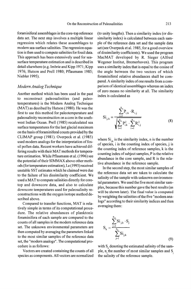
index is calculated as
n
"P. k ·R ..
L...J 1,
IJ
S·
_~i=~l========
Ij,k =
(8)
where Sij,k is the similarity index, n is the number
of species, i is the counting index of species, j is
the counting index of reference samples, k is the
counting index of subject samples, P is the relative
abundance in the core sample, and R is the relative abundance in the reference sample.
In the second step, the most similar samples of
the reference data set are taken to calculate the
salinity ofthe sample with unknown environmental parameters. We used the five most similar samples, because this number gave the best results (as
will be shown later). The final value is computed
by weighting the salinities of the five "modern analogs" according to their similarity indices and then
averaging them:
~Si'k ·S.
L... J,
J
S =..!.:i-::!l _ _ _
k
n,
ISij,k
j=l
(9)
with Sk denoting the estimated salinity ofthe sample, n, the number of most similar samples and Sj
the salinity of the reference sample.
213
foraminiferal assemblages in the core-top reference
data set. The next step involves a multiple linear
regression which relates these assemblages to
modern sea-surface salinities. The regression equation is then used to compute salinities for fossil data.
This approach has been extensively used for seasurface temperature estimation and is described in
detail elsewhere (e.g. Imbrie and Kipp 1971; Kipp
1976; Hutson and Prell 1980; pflaumann 1985;
Niebler 1995).
Modern Analog Technique
Another method which has been used in the past
to reconstruct paleosalinities (and paleotemperatures) is the Modern Analog Technique
(MAT) as desribed by Hutson (1980). He was the
first to use this method for paleotemperature and
paleosalinity reconstruction on a core in the southwest Indian Ocean. Prell (1985) recalculated sea
surface temperatures for the last glacial maximum
on the basis of foraminiferal counts provided by the
CLIMAP group (1981). Overpeck et al. (1985)
used modern analogs for the interpretation of fossil pollen data. Recent workers have achieved differing results with their MAT methods for temperature estimation. While pflaumann et al. (1996) see
the potential of their SIMMAX above other methods (for temperature estimation), Le (1993) received
unstable SST estimates which he claimed were due
to the failure of his dissimilarity coefficient. We
used a MAT to compute salinities directly for coretop and downcore data, and also to calculate
downcore temperatures used for paleosalinity reconstructions with the oxygen isotope method described above.
Compared to transfer functions, MAT is relatively simple in terms of its computational procedure. The relative abundances of planktonic
foraminifera of each sample are compared to the
counts of all samples in the modern reference data
set. The unknown environmental parameters are
then computed by averaging the parameters linked
to the most similar samples of the reference data
set, the "modern analogs". The computational procedure is as follows:
Vectors are created containing the counts of all
species as components. All vectors are normalized
(to unity lengths). Then a similarity index (or dissimilarity index) is calculated between each sample of the reference data set and the sample data
set (see Overpeck et al. 1985, for a good overview
of dissimilarity coefficients). We used the program
MacMAT developed by R. Sieger (Alfred
Wegener Institut, Bremerhaven). This program
uses a similarity index that is equal to the cosine of
the angle between the two vectors of which
foraminiferal relative abundances shall be compared. A similarity index of one results from a comparison of identical assemblages whereas an index
of zero means no similarity at all. The similarity
index is calculated as
n
"P. k ·R ..
L...J 1,
IJ
S·
_~i=~l========
Ij,k =
(8)
where Sij,k is the similarity index, n is the number
of species, i is the counting index of species, j is
the counting index of reference samples, k is the
counting index of subject samples, P is the relative
abundance in the core sample, and R is the relative abundance in the reference sample.
In the second step, the most similar samples of
the reference data set are taken to calculate the
salinity ofthe sample with unknown environmental parameters. We used the five most similar samples, because this number gave the best results (as
will be shown later). The final value is computed
by weighting the salinities of the five "modern analogs" according to their similarity indices and then
averaging them:
~Si'k ·S.
L... J,
J
S =..!.:i-::!l _ _ _
k
n,
ISij,k
j=l
(9)
with Sk denoting the estimated salinity ofthe sample, n, the number of most similar samples and Sj
the salinity of the reference sample.