

Storm Hazard Mitigation Structures 30.3 Shoreline Stabilization Structures 675
Part C | 30.3
d s : The mean water depth offshore at the toe of the
structure.
When the L s =L g ratio is large (long structure/small
gap) so that less wave energy reaches the shoreline
and/or when the Y=d s ratio is small (structure close to
shore in shallow water) tombolos form behind the structures which are called headland breakwaters. When the
opposite is true with these key ratios, more wave energy
reaches the shoreline to maintain long-shore sediment
transport processes and only salients are present behind
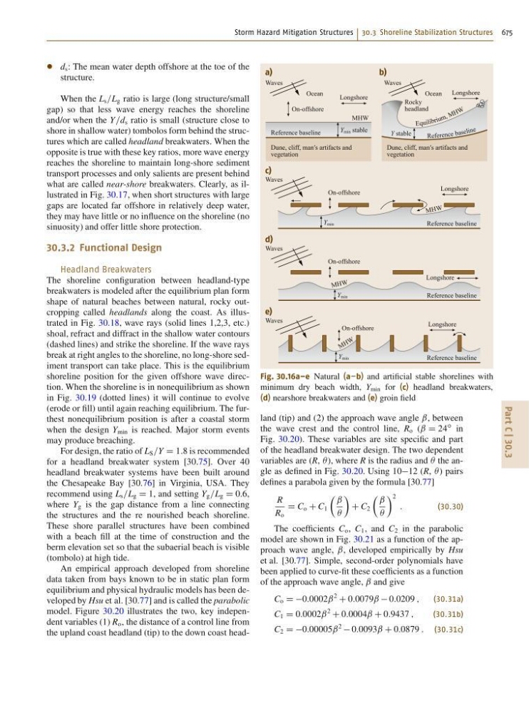
what are called near-shore breakwaters. Clearly, as illustrated in Fig. 30.17, when short structures with large
gaps are located far offshore in relatively deep water,
they may have little or no influence on the shoreline (no
sinuosity) and offer little shore protection.
30.3.2 Functional Design
Headland Breakwaters
The shoreline configuration between headland-type
breakwaters is modeled after the equilibrium plan form
shape of natural beaches between natural, rocky outcropping called headlands along the coast. As illustrated in Fig. 30.18, wave rays (solid lines 1,2,3, etc.)
shoal, refract and diffract in the shallow water contours
(dashed lines) and strike the shoreline. If the wave rays
break at right angles to the shoreline, no long-shore sediment transport can take place. This is the equilibrium
shoreline position for the given offshore wave direction. When the shoreline is in nonequilibrium as shown
in Fig. 30.19 (dotted lines) it will continue to evolve
(erode or fill) until again reaching equilibrium. The furthest nonequilibrium position is after a coastal storm
when the design Y min is reached. Major storm events
may produce breaching.
For design, the ratio of L S =Y D 1:8 is recommended
for a headland breakwater system [30.75]. Over 40
headland breakwater systems have been built around
the Chesapeake Bay [30.76] in Virginia, USA. They
recommend using L s =L g D 1, and setting Y g =L g D 0:6,
where Y g is the gap distance from a line connecting
the structures and the re nourished beach shoreline.
These shore parallel structures have been combined
with a beach fill at the time of construction and the
berm elevation set so that the subaerial beach is visible
(tombolo) at high tide.
An empirical approach developed from shoreline
data taken from bays known to be in static plan form
equilibrium and physical hydraulic models has been developed by Hsu et al. [30.77] and is called the parabolic
model. Figure 30.20 illustrates the two, key independent variables (1) R o , the distance of a control line from
the upland coast headland (tip) to the down coast headRefere nce ba se lin e
Equ ili br iu m , M H W
a)
c)
Waves
Y min stable
Y min
Reference baseline
Reference baseline
Dune, cliff, man′s artifacts and
vegetation
Longshore
On-offshore
On-offshore
MHW
M HW
Ocean
b)
Waves
Y stable
Dune, cliff, man′s artifacts and
vegetation
Longshore
Longshore
Rocky
headland
Ocean
Waves
d)
Y min
Reference baseline
On-offshore
M HW
Longshore
Waves
e)
Y min
Reference baseline
On-offshore
M H W
Longshore
Waves
Fig. 30.16a–e Natural (a–b) and artificial stable shorelines with
minimum dry beach width, Y min for (c) headland breakwaters,
(d) nearshore breakwaters and (e) groin field
land (tip) and (2) the approach wave angle ˇ, between
the wave crest and the control line, R o (ˇ D 24
ı in
Fig. 30.20). These variables are site specific and part
of the headland breakwater design. The two dependent
variables are (R,  ), where R is the radius and  the angle as defined in Fig. 30.20. Using 1012 (R,  ) pairs
defines a parabola given by the formula [30.77]
R
R o
D C o C C 1
 ˇ
Â
Ã
C C 2
 ˇ
Â
à 2
:
(30.30)
The coefficients C o , C 1 , and C 2 in the parabolic
model are shown in Fig. 30.21 as a function of the approach wave angle, ˇ, developed empirically by Hsu
et al. [30.77]. Simple, second-order polynomials have
been applied to curve-fit these coefficients as a function
of the approach wave angle, ˇ and give
C o D D0:0002ˇ
2
C 0:0079ˇ 0:0209 ;
(30.31a)
C 1 D 0:0002ˇ
2
C 0:0004ˇ C 0:9437 ;
(30.31b)
C 2 D D0:00005ˇ
2
0:0093ˇ C 0:0879 : (30.31c)