

Modeling of Coastal Morphological Processes 28.2 Principles of Process-Based Morphodynamic Modeling 615
Part C | 28.2
1000 m before groyne
500 m before groyne
at tip of groyne
500 m after groyne
1000 m after groyne
1500 m after groyne
0
500 1000 1500
Cum. erosion/sedimentation (m)
first 16 hours
2000 2500 3000
a) y (m)
x (m)
1500
1000
500
0
1
0.8
0.6
0.4
0.2
0
–0.2
–0.4
–0.6
–0.8
–1
0
500 1000 1500
Bed level (m)
after 3 years
2000 2500 3000
c) y (m)
x (m)
1500
1000
500
0
200
400
600
800
1000
1200
d) Transport through section (m
3
/s)
Time (yr)
10
0
10
–1
0
–2
–4
–6
–8
–10
–12
–14
–16
0
500 1000 1500
Total transport, magnitude: (m
3 /s/m)
initial
2000 2500 3000
b) y (m)
x (m)
1500
1000
500
0
0.004
0.0035
0.003
0.0025
0.002
0.0015
0.001
0.005
0
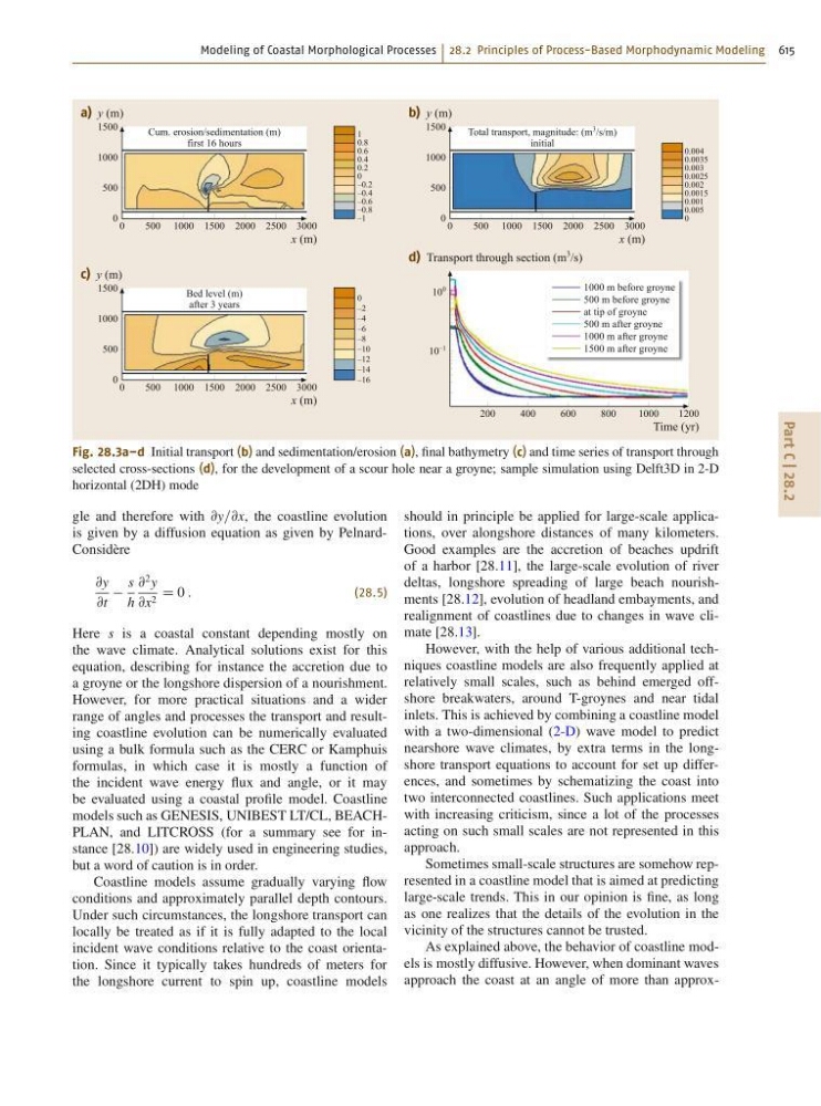
Fig. 28.3a–d Initial transport (b) and sedimentation/erosion (a), final bathymetry (c) and time series of transport through
selected cross-sections (d), for the development of a scour hole near a groyne; sample simulation using Delft3D in 2-D
horizontal (2DH) mode
gle and therefore with @y=@x, the coastline evolution
is given by a diffusion equation as given by PelnardConsidère
@y
@t
s
h
@
2 y
@x 2 D 0 :
(28.5)
Here s is a coastal constant depending mostly on
the wave climate. Analytical solutions exist for this
equation, describing for instance the accretion due to
a groyne or the longshore dispersion of a nourishment.
However, for more practical situations and a wider
range of angles and processes the transport and resulting coastline evolution can be numerically evaluated
using a bulk formula such as the CERC or Kamphuis
formulas, in which case it is mostly a function of
the incident wave energy flux and angle, or it may
be evaluated using a coastal profile model. Coastline
models such as GENESIS, UNIBEST LT/CL, BEACHPLAN, and LITCROSS (for a summary see for instance [28.10]) are widely used in engineering studies,
but a word of caution is in order.
Coastline models assume gradually varying flow
conditions and approximately parallel depth contours.
Under such circumstances, the longshore transport can
locally be treated as if it is fully adapted to the local
incident wave conditions relative to the coast orientation. Since it typically takes hundreds of meters for
the longshore current to spin up, coastline models
should in principle be applied for large-scale applications, over alongshore distances of many kilometers.
Good examples are the accretion of beaches updrift
of a harbor [28.11], the large-scale evolution of river
deltas, longshore spreading of large beach nourishments [28.12], evolution of headland embayments, and
realignment of coastlines due to changes in wave climate [28.13].
However, with the help of various additional techniques coastline models are also frequently applied at
relatively small scales, such as behind emerged offshore breakwaters, around T-groynes and near tidal
inlets. This is achieved by combining a coastline model
with a two-dimensional (2-D) wave model to predict
nearshore wave climates, by extra terms in the longshore transport equations to account for set up differences, and sometimes by schematizing the coast into
two interconnected coastlines. Such applications meet
with increasing criticism, since a lot of the processes
acting on such small scales are not represented in this
approach.
Sometimes small-scale structures are somehow represented in a coastline model that is aimed at predicting
large-scale trends. This in our opinion is fine, as long
as one realizes that the details of the evolution in the
vicinity of the structures cannot be trusted.
As explained above, the behavior of coastline models is mostly diffusive. However, when dominant waves
approach the coast at an angle of more than approx-