

Part C | 28.2
614 Part C Coastal Design
0 20 40 60 80 100 120 140 160 180 200 220
Bed level (m)
Distance from upstream 1-D (m)
0
–1
–2
–3
–4
–5
–6
–7
–8
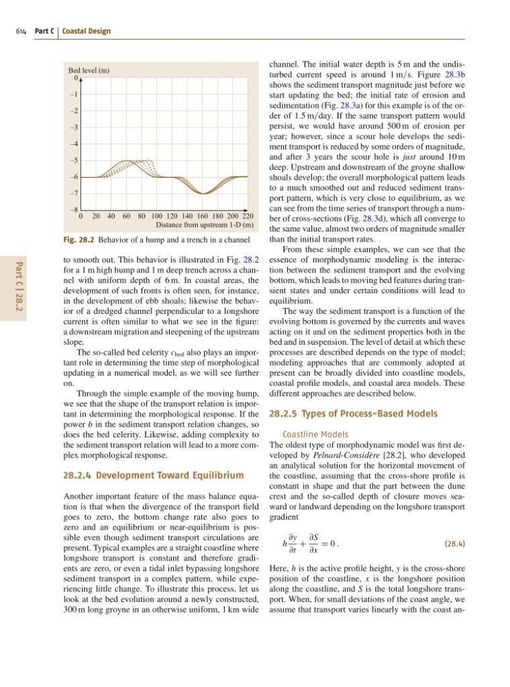
Fig. 28.2 Behavior of a hump and a trench in a channel
to smooth out. This behavior is illustrated in Fig. 28.2
for a 1 m high hump and 1 m deep trench across a channel with uniform depth of 6 m. In coastal areas, the
development of such fronts is often seen, for instance,
in the development of ebb shoals; likewise the behavior of a dredged channel perpendicular to a longshore
current is often similar to what we see in the figure:
a downstream migration and steepening of the upstream
slope.
The so-called bed celerity c bed also plays an important role in determining the time step of morphological
updating in a numerical model, as we will see further
on.
Through the simple example of the moving hump,
we see that the shape of the transport relation is important in determining the morphological response. If the
power b in the sediment transport relation changes, so
does the bed celerity. Likewise, adding complexity to
the sediment transport relation will lead to a more complex morphological response.
28.2.4 Development Toward Equilibrium
Another important feature of the mass balance equation is that when the divergence of the transport field
goes to zero, the bottom change rate also goes to
zero and an equilibrium or near-equilibrium is possible even though sediment transport circulations are
present. Typical examples are a straight coastline where
longshore transport is constant and therefore gradients are zero, or even a tidal inlet bypassing longshore
sediment transport in a complex pattern, while experiencing little change. To illustrate this process, let us
look at the bed evolution around a newly constructed,
300 m long groyne in an otherwise uniform, 1 km wide
channel. The initial water depth is 5 m and the undisturbed current speed is around 1 m=s. Figure 28.3b
shows the sediment transport magnitude just before we
start updating the bed; the initial rate of erosion and
sedimentation (Fig. 28.3a) for this example is of the order of 1:5 m=day. If the same transport pattern would
persist, we would have around 500 m of erosion per
year; however, since a scour hole develops the sediment transport is reduced by some orders of magnitude,
and after 3 years the scour hole is just around 10 m
deep. Upstream and downstream of the groyne shallow
shoals develop; the overall morphological pattern leads
to a much smoothed out and reduced sediment transport pattern, which is very close to equilibrium, as we
can see from the time series of transport through a number of cross-sections (Fig. 28.3d), which all converge to
the same value, almost two orders of magnitude smaller
than the initial transport rates.
From these simple examples, we can see that the
essence of morphodynamic modeling is the interaction between the sediment transport and the evolving
bottom, which leads to moving bed features during transient states and under certain conditions will lead to
equilibrium.
The way the sediment transport is a function of the
evolving bottom is governed by the currents and waves
acting on it and on the sediment properties both in the
bed and in suspension. The level of detail at which these
processes are described depends on the type of model;
modeling approaches that are commonly adopted at
present can be broadly divided into coastline models,
coastal profile models, and coastal area models. These
different approaches are described below.
28.2.5 Types of Process-Based Models
Coastline Models
The oldest type of morphodynamic model was first developed by Pelnard-Considère [28.2], who developed
an analytical solution for the horizontal movement of
the coastline, assuming that the cross-shore profile is
constant in shape and that the part between the dune
crest and the so-called depth of closure moves seaward or landward depending on the longshore transport
gradient
h
@y
@t
C
@S
@x
D 0 :
(28.4)
Here, h is the active profile height, y is the cross-shore
position of the coastline, x is the longshore position
along the coastline, and S is the total longshore transport. When, for small deviations of the coast angle, we
assume that transport varies linearly with the coast an-