

Part C | 27.4
606 Part C Coastal Design
31 32 33
t = 65 s
34 35
x (m)
36 37 38
a)
0.1
0
–0.1
–0.2
–0.3
–0.4
–0.5
31 32 33
t = 75 s
34 35
x (m)
36 37 38
b)
0.1
0
–0.1
–0.2
–0.3
–0.4
–0.5
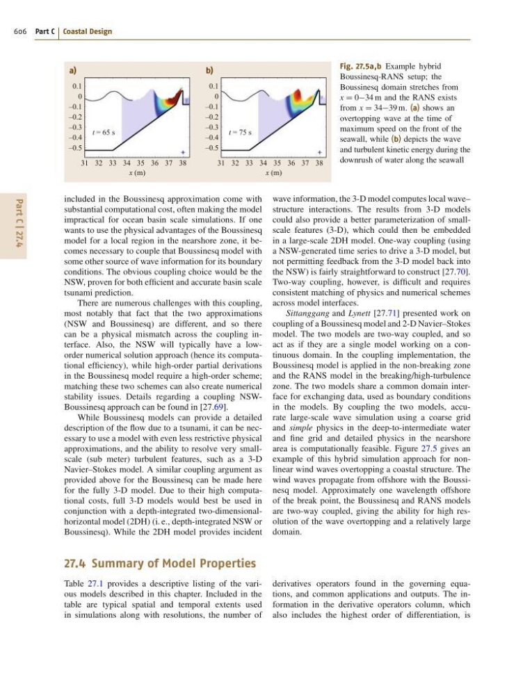
Fig. 27.5a,b Example hybrid
Boussinesq-RANS setup; the
Boussinesq domain stretches from
x D 034 m and the RANS exists
from x D 3439 m. (a) shows an
overtopping wave at the time of
maximum speed on the front of the
seawall, while (b) depicts the wave
and turbulent kinetic energy during the
downrush of water along the seawall
included in the Boussinesq approximation come with
substantial computational cost, often making the model
impractical for ocean basin scale simulations. If one
wants to use the physical advantages of the Boussinesq
model for a local region in the nearshore zone, it becomes necessary to couple that Boussinesq model with
some other source of wave information for its boundary
conditions. The obvious coupling choice would be the
NSW, proven for both efficient and accurate basin scale
tsunami prediction.
There are numerous challenges with this coupling,
most notably that fact that the two approximations
(NSW and Boussinesq) are different, and so there
can be a physical mismatch across the coupling interface. Also, the NSW will typically have a loworder numerical solution approach (hence its computational efficiency), while high-order partial derivations
in the Boussinesq model require a high-order scheme;
matching these two schemes can also create numerical
stability issues. Details regarding a coupling NSWBoussinesq approach can be found in [27.69].
While Boussinesq models can provide a detailed
description of the flow due to a tsunami, it can be necessary to use a model with even less restrictive physical
approximations, and the ability to resolve very smallscale (sub meter) turbulent features, such as a 3-D
Navier–Stokes model. A similar coupling argument as
provided above for the Boussinesq can be made here
for the fully 3-D model. Due to their high computational costs, full 3-D models would best be used in
conjunction with a depth-integrated two-dimensionalhorizontal model (2DH) (i. e., depth-integrated NSW or
Boussinesq). While the 2DH model provides incident
wave information, the 3-D model computes local wave–
structure interactions. The results from 3-D models
could also provide a better parameterization of smallscale features (3-D), which could then be embedded
in a large-scale 2DH model. One-way coupling (using
a NSW-generated time series to drive a 3-D model, but
not permitting feedback from the 3-D model back into
the NSW) is fairly straightforward to construct [27.70].
Two-way coupling, however, is difficult and requires
consistent matching of physics and numerical schemes
across model interfaces.
Sittanggang and Lynett [27.71] presented work on
coupling of a Boussinesq model and 2-D Navier–Stokes
model. The two models are two-way coupled, and so
act as if they are a single model working on a continuous domain. In the coupling implementation, the
Boussinesq model is applied in the non-breaking zone
and the RANS model in the breaking/high-turbulence
zone. The two models share a common domain interface for exchanging data, used as boundary conditions
in the models. By coupling the two models, accurate large-scale wave simulation using a coarse grid
and simple physics in the deep-to-intermediate water
and fine grid and detailed physics in the nearshore
area is computationally feasible. Figure 27.5 gives an
example of this hybrid simulation approach for nonlinear wind waves overtopping a coastal structure. The
wind waves propagate from offshore with the Boussinesq model. Approximately one wavelength offshore
of the break point, the Boussinesq and RANS models
are two-way coupled, giving the ability for high resolution of the wave overtopping and a relatively large
domain.
27.4 Summary of Model Properties
Table 27.1 provides a descriptive listing of the various models described in this chapter. Included in the
table are typical spatial and temporal extents used
in simulations along with resolutions, the number of
derivatives operators found in the governing equations, and common applications and outputs. The information in the derivative operators column, which
also includes the highest order of differentiation, is