

Autonomy: Risk Assessment 24.5 Risk of Loss 539
Part B | 24.5
process so they can share their knowledge and allow
persuasive arguments to change their views, and help
them to generate a consensus distribution [24.41]. This
approach is often more transparent and more immune
to criticism than mathematical aggregation methods.
A behavioral expert judgment elicitation was conducted to build a risk model for two ISE Explorer
AUVs, operated by Defence Research Development
Canada (DRDC) [24.19]. As these vehicles were to be
used on data gathering of national importance in the
high Arctic [24.42], a transparent and justifiable process
was needed for how the risk of vehicle loss was evaluated; hence a behavioral aggregation approach was
taken. Analysis of the outcomes of the discussions central to behavioral aggregation showed that there were
seven classes of fault assessments:
Assessments where the panel reached unanimity
that the fault would inevitably lead to loss under ice,
which included five faults where experts set all parameters of the distribution to 1.
Assessments where the panel reached unanimity
that the fault would have no impact at all on survivability, such as failure of a component or subsystem
that would not be present for the Arctic.
Assessments for faults where the experts considered
that the phase of the mission may affect the consequence. This class of faults, typified by a failure
in the vehicle control computer, resulted in vigorous discussion by the experts on the probability of
loss, as some experts considered the outcome to be
strongly dependent on the phase of the mission during which the fault occurred.
Assessments of faults where individual experts
shared particular insights affecting the aggregated
outcome.
Assessments where there was an agreement that the
fault leads to a wide range of probability of loss.
Assessments of faults that provided insights into
instances of where a fault implied a consequential
vulnerability.
Assessments where the panel reached an agreement
to use heuristic shortcuts. The group agreed collectively that they would spend little time on those
faults that had a very low, but nonzero, consequence
for the risk of loss. For these, they agreed on a standard distribution with a lower limit of 0, a median
of 6:2 10
8 , and an upper limit of 10
6 .
A novel aspect of this study was the quantification
of the risk mitigation activities. For each fault, experts
were asked to assess of the impact of the risk mitigation plan, setting P M to 0 if they believed that the
mitigation strategy would not mitigate the fault and
to 1 if the mitigation plan would completely mitigate
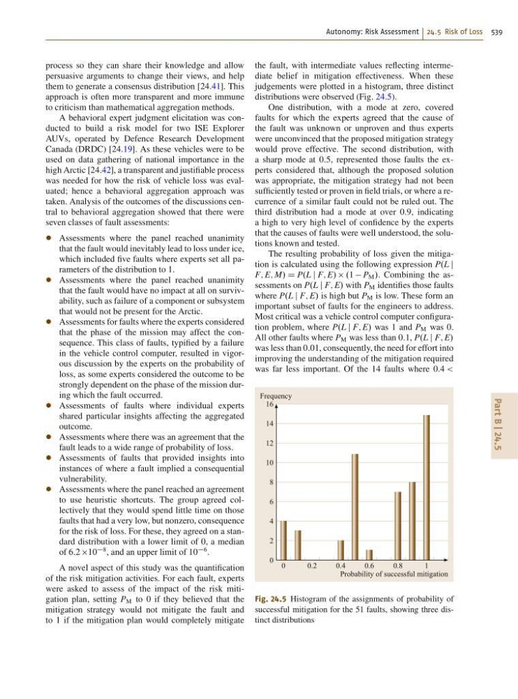
the fault, with intermediate values reflecting intermediate belief in mitigation effectiveness. When these
judgements were plotted in a histogram, three distinct
distributions were observed (Fig. 24.5).
One distribution, with a mode at zero, covered
faults for which the experts agreed that the cause of
the fault was unknown or unproven and thus experts
were unconvinced that the proposed mitigation strategy
would prove effective. The second distribution, with
a sharp mode at 0:5, represented those faults the experts considered that, although the proposed solution
was appropriate, the mitigation strategy had not been
sufficiently tested or proven in field trials, or where a recurrence of a similar fault could not be ruled out. The
third distribution had a mode at over 0:9, indicating
a high to very high level of confidence by the experts
that the causes of faults were well understood, the solutions known and tested.
The resulting probability of loss given the mitigation is calculated using the following expression P.L j
F; E; M/ D P.L j F; E/ .1 P M /. Combining the assessments on P.L j F; E/ with P M identifies those faults
where P.L j F; E/ is high but P M is low. These form an
important subset of faults for the engineers to address.
Most critical was a vehicle control computer configuration problem, where P.L j F; E/ was 1 and P M was 0.
All other faults where P M was less than 0:1, P.L j F; E/
was less than 0:01, consequently, the need for effort into
improving the understanding of the mitigation required
was far less important. Of the 14 faults where 0:4 <
0
0.2
0.4
0.6
0.8
1
Frequency
Probability of successful mitigation
16
14
12
10
8
6
4
2
0
Fig. 24.5 Histogram of the assignments of probability of
successful mitigation for the 51 faults, showing three distinct distributions