

Part B | 21.3
494 Part B Autonomous Ocean Vehicles, Subsystems and Control
True solution
D.O. solution
Adaptive observations
Fixed observations
Adaptive observations
Fixed observations
Time passed: 10. Time until next observation: 0.25
a)
20
15
10
5
0
–5
–10
–15
–20
b)
c)
0
1
2
3
4
5
6
7
8
9
1 0
Time
1.5
1
0.5
0
–10
0
10
Mode number 1
0.4
0.2
0
–5
0
5
Mode number 2
0.4
0.2
0
–5
0
5
Mode number 3
Root mean square error (RMSE)
1
0.5
0
–10
0
–5
2
0
2
0
5
Mode number 4
1
0.5
0
–2
4
Mode number 5
2
1
0
–2
0
2
Mode number 6
2
1
0
–2
4
Mode number 7
2
1
0
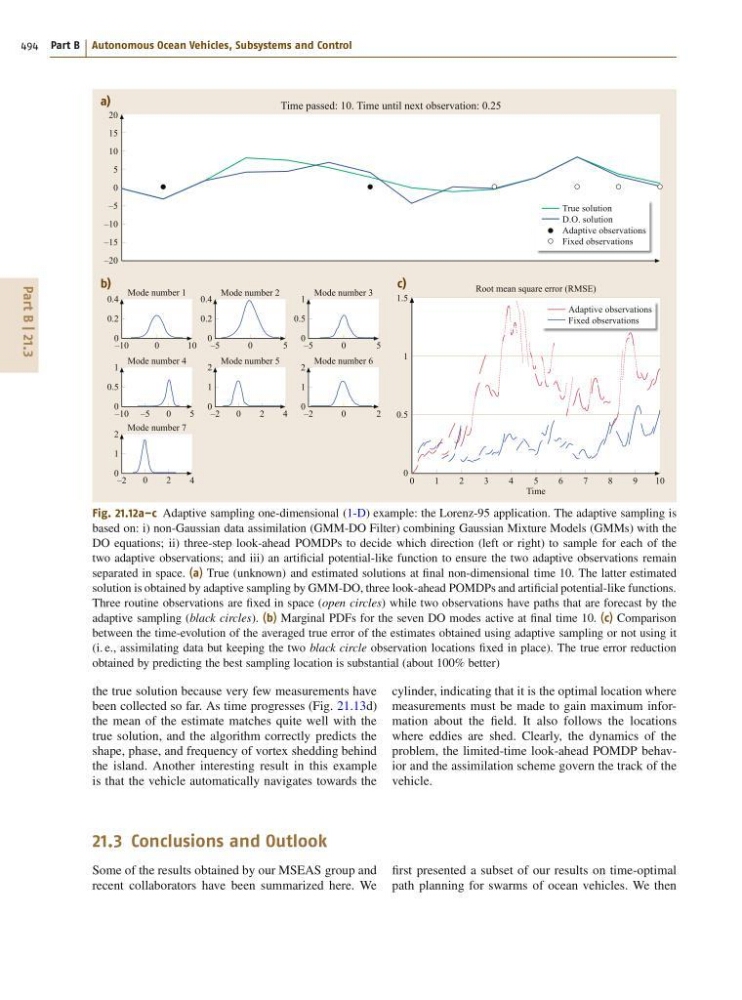
Fig. 21.12a–c Adaptive sampling one-dimensional (1-D) example: the Lorenz-95 application. The adaptive sampling is
based on: i) non-Gaussian data assimilation (GMM-DO Filter) combining Gaussian Mixture Models (GMMs) with the
DO equations; ii) three-step look-ahead POMDPs to decide which direction (left or right) to sample for each of the
two adaptive observations; and iii) an artificial potential-like function to ensure the two adaptive observations remain
separated in space. (a) True (unknown) and estimated solutions at final non-dimensional time 10. The latter estimated
solution is obtained by adaptive sampling by GMM-DO, three look-ahead POMDPs and artificial potential-like functions.
Three routine observations are fixed in space (open circles) while two observations have paths that are forecast by the
adaptive sampling (black circles). (b) Marginal PDFs for the seven DO modes active at final time 10. (c) Comparison
between the time-evolution of the averaged true error of the estimates obtained using adaptive sampling or not using it
(i. e., assimilating data but keeping the two black circle observation locations fixed in place). The true error reduction
obtained by predicting the best sampling location is substantial (about 100% better)
the true solution because very few measurements have
been collected so far. As time progresses (Fig. 21.13d)
the mean of the estimate matches quite well with the
true solution, and the algorithm correctly predicts the
shape, phase, and frequency of vortex shedding behind
the island. Another interesting result in this example
is that the vehicle automatically navigates towards the
cylinder, indicating that it is the optimal location where
measurements must be made to gain maximum information about the field. It also follows the locations
where eddies are shed. Clearly, the dynamics of the
problem, the limited-time look-ahead POMDP behavior and the assimilation scheme govern the track of the
vehicle.
21.3 Conclusions and Outlook
Some of the results obtained by our MSEAS group and
recent collaborators have been summarized here. We
first presented a subset of our results on time-optimal
path planning for swarms of ocean vehicles. We then
494 Part B Autonomous Ocean Vehicles, Subsystems and Control
True solution
D.O. solution
Adaptive observations
Fixed observations
Adaptive observations
Fixed observations
Time passed: 10. Time until next observation: 0.25
a)
20
15
10
5
0
–5
–10
–15
–20
b)
c)
0
1
2
3
4
5
6
7
8
9
1 0
Time
1.5
1
0.5
0
–10
0
10
Mode number 1
0.4
0.2
0
–5
0
5
Mode number 2
0.4
0.2
0
–5
0
5
Mode number 3
Root mean square error (RMSE)
1
0.5
0
–10
0
–5
2
0
2
0
5
Mode number 4
1
0.5
0
–2
4
Mode number 5
2
1
0
–2
0
2
Mode number 6
2
1
0
–2
4
Mode number 7
2
1
0
Fig. 21.12a–c Adaptive sampling one-dimensional (1-D) example: the Lorenz-95 application. The adaptive sampling is
based on: i) non-Gaussian data assimilation (GMM-DO Filter) combining Gaussian Mixture Models (GMMs) with the
DO equations; ii) three-step look-ahead POMDPs to decide which direction (left or right) to sample for each of the
two adaptive observations; and iii) an artificial potential-like function to ensure the two adaptive observations remain
separated in space. (a) True (unknown) and estimated solutions at final non-dimensional time 10. The latter estimated
solution is obtained by adaptive sampling by GMM-DO, three look-ahead POMDPs and artificial potential-like functions.
Three routine observations are fixed in space (open circles) while two observations have paths that are forecast by the
adaptive sampling (black circles). (b) Marginal PDFs for the seven DO modes active at final time 10. (c) Comparison
between the time-evolution of the averaged true error of the estimates obtained using adaptive sampling or not using it
(i. e., assimilating data but keeping the two black circle observation locations fixed in place). The true error reduction
obtained by predicting the best sampling location is substantial (about 100% better)
the true solution because very few measurements have
been collected so far. As time progresses (Fig. 21.13d)
the mean of the estimate matches quite well with the
true solution, and the algorithm correctly predicts the
shape, phase, and frequency of vortex shedding behind
the island. Another interesting result in this example
is that the vehicle automatically navigates towards the
cylinder, indicating that it is the optimal location where
measurements must be made to gain maximum information about the field. It also follows the locations
where eddies are shed. Clearly, the dynamics of the
problem, the limited-time look-ahead POMDP behavior and the assimilation scheme govern the track of the
vehicle.
21.3 Conclusions and Outlook
Some of the results obtained by our MSEAS group and
recent collaborators have been summarized here. We
first presented a subset of our results on time-optimal
path planning for swarms of ocean vehicles. We then