

Science of Autonomy for Swarms of Ocean Vehicles 21.2 Adaptive Sampling for Swarms of Ocean Vehicles 493
Part B | 21.2
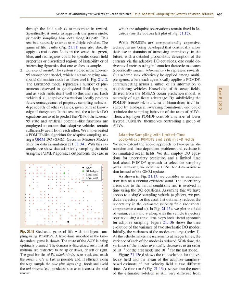
through the field such as to maximize its reward.
Specifically, it seeks to approach the green circle,
primarily sampling blue dots along its path. This
test bed naturally extends to multiple vehicles. The
game of life results (Fig. 21.11) may also directly
apply to real ocean fields in the sense that green,
blue, and red regions could be specific ocean field
properties or discretized regions of instability or of
interesting dynamics that one wishes to sample.
2. Lorenz-95 model: The system studied is the Lorenz95 atmospheric model, which is a time-varying onespatial dimension model, as illustrated in Fig. 21.12.
The Lorenz-95 model replicates a number of phenomena observed in geophysical fluid dynamics,
and as such lends itself well to this analysis. Each
vehicle (i. e., adaptive observation) locally predicts
future consequences of proposed sampling paths, independently of other vehicles, given current knowledge of the system. In this test bed, the adaptive DO
equations are used to predict the PDF of the Lorenz95 state and artificial potential-like functions are
employed to ensure that adaptive vehicles remain
sufficiently apart from each other. We implemented
a POMDP-like algorithm for adaptive sampling, using a GMM-DO (GMM: Gaussian Mixture Model)
filter for data assimilation [21.33, 34]. With this example, we show that adaptively sampling the field
using the POMDP approach outperforms the case in
AUV
Global goal
Local goal
Local cost
Fig. 21.11 Stochastic game of life with intelligent sampling using POMDPs. A fixed-time snapshot in the timedependent game is shown. The route of the AUV is being
optimally planned. The domain is discretized such that all
motions are restricted to be up or down, or left or right.
The goal for the AUV, black circle, is to track and reach
the green circle as fast as possible and, if efficient along
the way, sample the blue plus signs (e.g., food) and avoid
the red crosses (e.g., predators), so as to increase the total
reward
which the adaptive observations remain fixed in location (see the bottom left plot of Fig. 21.12).
While POMDPs are computationally expensive,
techniques are being developed that continually allow
their use in domains of increasing complexity. In the
future, with a detailed probabilistic description of the
currents via the adaptive DO equations, one could derive novel metrics using information theoretic measures
(specifically mutual information) to represent rewards.
Our scheme may effectively be applied among multiple agents, where each agent locally applies a POMDP,
communicating across a subset of its information to
neighboring vehicles. Knowledge of the ocean fields,
derived from the MSEAS ocean prediction model, is
naturally of significant advantage. By subdividing the
POMDP framework into a set of hierarchies, itself inspired by biological swarming formations, one could
optimize the sampling behavior of the team of AUVs.
Then, a top layer POMDP controls a number of lower
layered POMDPs, themselves controlling a group of
AUVs.
Adaptive Sampling with Limited-Time
Look-Ahead POMDPs and ESSE in 2-D Fields
We now extend the above approach to two-spatial dimension and time-dependent problems and evaluate it
on simulated ocean fields. We still employ DO equations for uncertainty prediction and a limited time
look-ahead POMDP approach to select the sampling
paths. However, we now use ESSE for data assimilation instead of the GMM update.
As shown in Fig. 21.13, we consider an uncertain
flow behind a circular cylinder/island. The uncertainty
arises due to the initial conditions and is evolved in
time using the DO equations. Assuming that we have
access to a single sampling vehicle (a glider), we predict a trajectory for this asset that optimally reduces the
uncertainty in the estimated velocity field (horizontal
components: u and v ). In Fig. 21.13a, we plot the field
of variance in u and v along with the vehicle trajectory
obtained using a three-time-steps look-ahead approach
for adaptive sampling. Figure 21.13b shows the time
evolution of the variance of two stochastic DO modes.
Initially, the variances of the modes are large (order 1).
As the vehicle makes measurements at integer times, the
variance of each of the modes is reduced. With time, the
variance of the modes eventually decreases to an order
of 10
1 for the first mode and 10
5 for the last mode.
Figure 21.13c,d shows the true solution for the velocity field and the mean of the adaptive-samplingbased estimate of that velocity field at two different
times. At time t D 6 (Fig. 21.13c), we see that the mean
of the estimated solution is still very different from
Part B | 21.2
through the field such as to maximize its reward.
Specifically, it seeks to approach the green circle,
primarily sampling blue dots along its path. This
test bed naturally extends to multiple vehicles. The
game of life results (Fig. 21.11) may also directly
apply to real ocean fields in the sense that green,
blue, and red regions could be specific ocean field
properties or discretized regions of instability or of
interesting dynamics that one wishes to sample.
2. Lorenz-95 model: The system studied is the Lorenz95 atmospheric model, which is a time-varying onespatial dimension model, as illustrated in Fig. 21.12.
The Lorenz-95 model replicates a number of phenomena observed in geophysical fluid dynamics,
and as such lends itself well to this analysis. Each
vehicle (i. e., adaptive observation) locally predicts
future consequences of proposed sampling paths, independently of other vehicles, given current knowledge of the system. In this test bed, the adaptive DO
equations are used to predict the PDF of the Lorenz95 state and artificial potential-like functions are
employed to ensure that adaptive vehicles remain
sufficiently apart from each other. We implemented
a POMDP-like algorithm for adaptive sampling, using a GMM-DO (GMM: Gaussian Mixture Model)
filter for data assimilation [21.33, 34]. With this example, we show that adaptively sampling the field
using the POMDP approach outperforms the case in
AUV
Global goal
Local goal
Local cost
Fig. 21.11 Stochastic game of life with intelligent sampling using POMDPs. A fixed-time snapshot in the timedependent game is shown. The route of the AUV is being
optimally planned. The domain is discretized such that all
motions are restricted to be up or down, or left or right.
The goal for the AUV, black circle, is to track and reach
the green circle as fast as possible and, if efficient along
the way, sample the blue plus signs (e.g., food) and avoid
the red crosses (e.g., predators), so as to increase the total
reward
which the adaptive observations remain fixed in location (see the bottom left plot of Fig. 21.12).
While POMDPs are computationally expensive,
techniques are being developed that continually allow
their use in domains of increasing complexity. In the
future, with a detailed probabilistic description of the
currents via the adaptive DO equations, one could derive novel metrics using information theoretic measures
(specifically mutual information) to represent rewards.
Our scheme may effectively be applied among multiple agents, where each agent locally applies a POMDP,
communicating across a subset of its information to
neighboring vehicles. Knowledge of the ocean fields,
derived from the MSEAS ocean prediction model, is
naturally of significant advantage. By subdividing the
POMDP framework into a set of hierarchies, itself inspired by biological swarming formations, one could
optimize the sampling behavior of the team of AUVs.
Then, a top layer POMDP controls a number of lower
layered POMDPs, themselves controlling a group of
AUVs.
Adaptive Sampling with Limited-Time
Look-Ahead POMDPs and ESSE in 2-D Fields
We now extend the above approach to two-spatial dimension and time-dependent problems and evaluate it
on simulated ocean fields. We still employ DO equations for uncertainty prediction and a limited time
look-ahead POMDP approach to select the sampling
paths. However, we now use ESSE for data assimilation instead of the GMM update.
As shown in Fig. 21.13, we consider an uncertain
flow behind a circular cylinder/island. The uncertainty
arises due to the initial conditions and is evolved in
time using the DO equations. Assuming that we have
access to a single sampling vehicle (a glider), we predict a trajectory for this asset that optimally reduces the
uncertainty in the estimated velocity field (horizontal
components: u and v ). In Fig. 21.13a, we plot the field
of variance in u and v along with the vehicle trajectory
obtained using a three-time-steps look-ahead approach
for adaptive sampling. Figure 21.13b shows the time
evolution of the variance of two stochastic DO modes.
Initially, the variances of the modes are large (order 1).
As the vehicle makes measurements at integer times, the
variance of each of the modes is reduced. With time, the
variance of the modes eventually decreases to an order
of 10
1 for the first mode and 10
5 for the last mode.
Figure 21.13c,d shows the true solution for the velocity field and the mean of the adaptive-samplingbased estimate of that velocity field at two different
times. At time t D 6 (Fig. 21.13c), we see that the mean
of the estimated solution is still very different from