

Part B | 21.2
492 Part B Autonomous Ocean Vehicles, Subsystems and Control
–150 –100 –50
0
50
100
150
Distance N/S (km)
Distance E/W (km)
100
50
0
–50
–100
–150
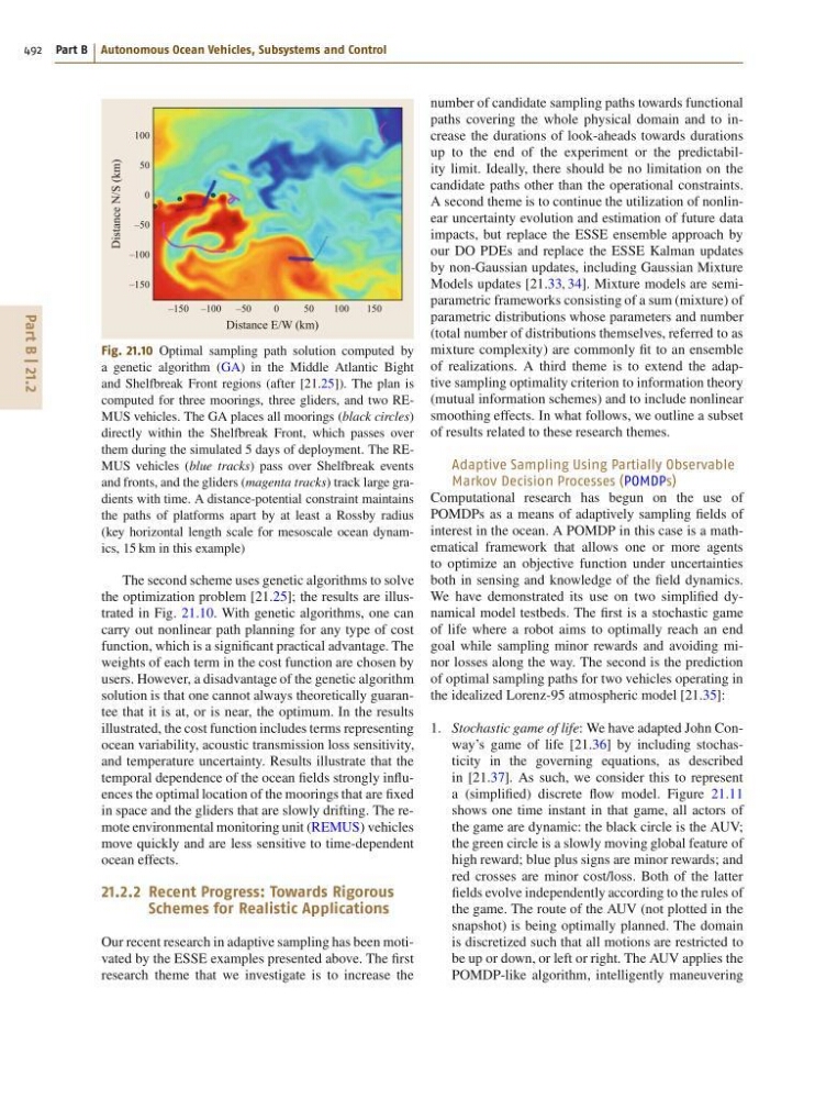
Fig. 21.10 Optimal sampling path solution computed by
a genetic algorithm (GA) in the Middle Atlantic Bight
and Shelfbreak Front regions (after [21.25]). The plan is
computed for three moorings, three gliders, and two REMUS vehicles. The GA places all moorings (black circles)
directly within the Shelfbreak Front, which passes over
them during the simulated 5 days of deployment. The REMUS vehicles (blue tracks) pass over Shelfbreak events
and fronts, and the gliders (magenta tracks) track large gradients with time. A distance-potential constraint maintains
the paths of platforms apart by at least a Rossby radius
(key horizontal length scale for mesoscale ocean dynamics, 15 km in this example)
The second scheme uses genetic algorithms to solve
the optimization problem [21.25]; the results are illustrated in Fig. 21.10. With genetic algorithms, one can
carry out nonlinear path planning for any type of cost
function, which is a significant practical advantage. The
weights of each term in the cost function are chosen by
users. However, a disadvantage of the genetic algorithm
solution is that one cannot always theoretically guarantee that it is at, or is near, the optimum. In the results
illustrated, the cost function includes terms representing
ocean variability, acoustic transmission loss sensitivity,
and temperature uncertainty. Results illustrate that the
temporal dependence of the ocean fields strongly influences the optimal location of the moorings that are fixed
in space and the gliders that are slowly drifting. The remote environmental monitoring unit (REMUS) vehicles
move quickly and are less sensitive to time-dependent
ocean effects.
21.2.2 Recent Progress: Towards Rigorous
Schemes for Realistic Applications
Our recent research in adaptive sampling has been motivated by the ESSE examples presented above. The first
research theme that we investigate is to increase the
number of candidate sampling paths towards functional
paths covering the whole physical domain and to increase the durations of look-aheads towards durations
up to the end of the experiment or the predictability limit. Ideally, there should be no limitation on the
candidate paths other than the operational constraints.
A second theme is to continue the utilization of nonlinear uncertainty evolution and estimation of future data
impacts, but replace the ESSE ensemble approach by
our DO PDEs and replace the ESSE Kalman updates
by non-Gaussian updates, including Gaussian Mixture
Models updates [21.33, 34]. Mixture models are semiparametric frameworks consisting of a sum (mixture) of
parametric distributions whose parameters and number
(total number of distributions themselves, referred to as
mixture complexity) are commonly fit to an ensemble
of realizations. A third theme is to extend the adaptive sampling optimality criterion to information theory
(mutual information schemes) and to include nonlinear
smoothing effects. In what follows, we outline a subset
of results related to these research themes.
Adaptive Sampling Using Partially Observable
Markov Decision Processes (POMDPs)
Computational research has begun on the use of
POMDPs as a means of adaptively sampling fields of
interest in the ocean. A POMDP in this case is a mathematical framework that allows one or more agents
to optimize an objective function under uncertainties
both in sensing and knowledge of the field dynamics.
We have demonstrated its use on two simplified dynamical model testbeds. The first is a stochastic game
of life where a robot aims to optimally reach an end
goal while sampling minor rewards and avoiding minor losses along the way. The second is the prediction
of optimal sampling paths for two vehicles operating in
the idealized Lorenz-95 atmospheric model [21.35]:
1. Stochastic game of life: We have adapted John Conway’s game of life [21.36] by including stochasticity in the governing equations, as described
in [21.37]. As such, we consider this to represent
a (simplified) discrete flow model. Figure 21.11
shows one time instant in that game, all actors of
the game are dynamic: the black circle is the AUV;
the green circle is a slowly moving global feature of
high reward; blue plus signs are minor rewards; and
red crosses are minor cost/loss. Both of the latter
fields evolve independently according to the rules of
the game. The route of the AUV (not plotted in the
snapshot) is being optimally planned. The domain
is discretized such that all motions are restricted to
be up or down, or left or right. The AUV applies the
POMDP-like algorithm, intelligently maneuvering
492 Part B Autonomous Ocean Vehicles, Subsystems and Control
–150 –100 –50
0
50
100
150
Distance N/S (km)
Distance E/W (km)
100
50
0
–50
–100
–150
Fig. 21.10 Optimal sampling path solution computed by
a genetic algorithm (GA) in the Middle Atlantic Bight
and Shelfbreak Front regions (after [21.25]). The plan is
computed for three moorings, three gliders, and two REMUS vehicles. The GA places all moorings (black circles)
directly within the Shelfbreak Front, which passes over
them during the simulated 5 days of deployment. The REMUS vehicles (blue tracks) pass over Shelfbreak events
and fronts, and the gliders (magenta tracks) track large gradients with time. A distance-potential constraint maintains
the paths of platforms apart by at least a Rossby radius
(key horizontal length scale for mesoscale ocean dynamics, 15 km in this example)
The second scheme uses genetic algorithms to solve
the optimization problem [21.25]; the results are illustrated in Fig. 21.10. With genetic algorithms, one can
carry out nonlinear path planning for any type of cost
function, which is a significant practical advantage. The
weights of each term in the cost function are chosen by
users. However, a disadvantage of the genetic algorithm
solution is that one cannot always theoretically guarantee that it is at, or is near, the optimum. In the results
illustrated, the cost function includes terms representing
ocean variability, acoustic transmission loss sensitivity,
and temperature uncertainty. Results illustrate that the
temporal dependence of the ocean fields strongly influences the optimal location of the moorings that are fixed
in space and the gliders that are slowly drifting. The remote environmental monitoring unit (REMUS) vehicles
move quickly and are less sensitive to time-dependent
ocean effects.
21.2.2 Recent Progress: Towards Rigorous
Schemes for Realistic Applications
Our recent research in adaptive sampling has been motivated by the ESSE examples presented above. The first
research theme that we investigate is to increase the
number of candidate sampling paths towards functional
paths covering the whole physical domain and to increase the durations of look-aheads towards durations
up to the end of the experiment or the predictability limit. Ideally, there should be no limitation on the
candidate paths other than the operational constraints.
A second theme is to continue the utilization of nonlinear uncertainty evolution and estimation of future data
impacts, but replace the ESSE ensemble approach by
our DO PDEs and replace the ESSE Kalman updates
by non-Gaussian updates, including Gaussian Mixture
Models updates [21.33, 34]. Mixture models are semiparametric frameworks consisting of a sum (mixture) of
parametric distributions whose parameters and number
(total number of distributions themselves, referred to as
mixture complexity) are commonly fit to an ensemble
of realizations. A third theme is to extend the adaptive sampling optimality criterion to information theory
(mutual information schemes) and to include nonlinear
smoothing effects. In what follows, we outline a subset
of results related to these research themes.
Adaptive Sampling Using Partially Observable
Markov Decision Processes (POMDPs)
Computational research has begun on the use of
POMDPs as a means of adaptively sampling fields of
interest in the ocean. A POMDP in this case is a mathematical framework that allows one or more agents
to optimize an objective function under uncertainties
both in sensing and knowledge of the field dynamics.
We have demonstrated its use on two simplified dynamical model testbeds. The first is a stochastic game
of life where a robot aims to optimally reach an end
goal while sampling minor rewards and avoiding minor losses along the way. The second is the prediction
of optimal sampling paths for two vehicles operating in
the idealized Lorenz-95 atmospheric model [21.35]:
1. Stochastic game of life: We have adapted John Conway’s game of life [21.36] by including stochasticity in the governing equations, as described
in [21.37]. As such, we consider this to represent
a (simplified) discrete flow model. Figure 21.11
shows one time instant in that game, all actors of
the game are dynamic: the black circle is the AUV;
the green circle is a slowly moving global feature of
high reward; blue plus signs are minor rewards; and
red crosses are minor cost/loss. Both of the latter
fields evolve independently according to the rules of
the game. The route of the AUV (not plotted in the
snapshot) is being optimally planned. The domain
is discretized such that all motions are restricted to
be up or down, or left or right. The AUV applies the
POMDP-like algorithm, intelligently maneuvering