

Science of Autonomy for Swarms of Ocean Vehicles 21.2 Adaptive Sampling for Swarms of Ocean Vehicles 491
Part B | 21.2
0
0.5
1
Range (km)
Depth (m)
1.5
2
a) 0
10
20
30
40
50
60
70
1540
1535
1530
1525
1520
1515
1510
(m/s)
0
0.5
1
1.5
2
b) 0
20
40
60
1540
1530
1520
1510
1500
1490
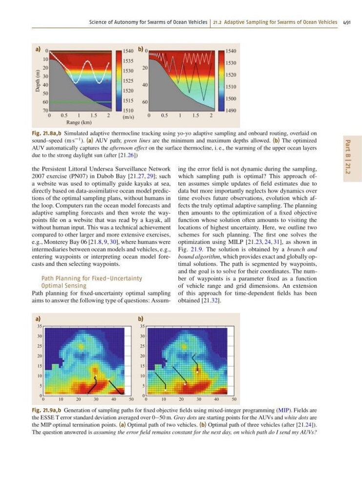
Fig. 21.8a,b Simulated adaptive thermocline tracking using yo-yo adaptive sampling and onboard routing, overlaid on
sound–speed (m s
1 ). (a) AUV path; green lines are the minimum and maximum depths allowed. (b) The optimized
AUV automatically captures the afternoon effect on the surface thermocline, i. e., the warming of the upper ocean layers
due to the strong daylight sun (after [21.26])
the Persistent Littoral Undersea Surveillance Network
2007 exercise (PN07) in Dabob Bay [21.27, 29]; such
a website was used to optimally guide kayaks at sea,
directly based on data-assimilative ocean model predictions of the optimal sampling plans, without humans in
the loop. Computers ran the ocean model forecasts and
adaptive sampling forecasts and then wrote the waypoints file on a website that was read by a kayak, all
without human input. This was a technical achievement
compared to other larger and more extensive exercises,
e.g., Monterey Bay 06 [21.8, 9, 30], where humans were
intermediaries between ocean models and vehicles, e.g.,
entering waypoints or interpreting ocean model forecasts and then selecting waypoints.
Path Planning for Fixed-Uncertainty
Optimal Sensing
Path planning for fixed-uncertainty optimal sampling
aims to answer the following type of questions: Assum0
1 0
2 0
3 0
4 0
5 0
a)
35
30
25
20
15
10
5
0
0
1 0
2 0
3 0
4 0
5 0
35
30
25
20
15
10
5
0
b)
Fig. 21.9a,b Generation of sampling paths for fixed objective fields using mixed-integer programming (MIP). Fields are
the ESSE T error standard deviation averaged over 050 m. Gray dots are starting points for the AUVs and white dots are
the MIP optimal termination points. (a) Optimal path of two vehicles. (b) Optimal path of three vehicles (after [21.24]).
The question answered is assuming the error field remains constant for the next day, on which path do I send my AUVs?
ing the error field is not dynamic during the sampling,
which sampling path is optimal? This approach often assumes simple updates of field estimates due to
data but more importantly neglects how dynamics over
time evolves future observations, evolution which affects the truly optimal adaptive sampling. The planning
then amounts to the optimization of a fixed objective
function whose solution often amounts to visiting the
locations of highest uncertainty. Here, we outline two
schemes for such planning. The first one solves the
optimization using MILP [21.23, 24, 31], as shown in
Fig. 21.9. The solution is obtained by a branch and
bound algorithm, which provides exact and globally optimal solutions. The path is segmented by waypoints,
and the goal is to solve for their coordinates. The number of waypoints is a parameter fixed as a function
of vehicle range and grid dimensions. An extension
of this approach for time-dependent fields has been
obtained [21.32].
Part B | 21.2
0
0.5
1
Range (km)
Depth (m)
1.5
2
a) 0
10
20
30
40
50
60
70
1540
1535
1530
1525
1520
1515
1510
(m/s)
0
0.5
1
1.5
2
b) 0
20
40
60
1540
1530
1520
1510
1500
1490
Fig. 21.8a,b Simulated adaptive thermocline tracking using yo-yo adaptive sampling and onboard routing, overlaid on
sound–speed (m s
1 ). (a) AUV path; green lines are the minimum and maximum depths allowed. (b) The optimized
AUV automatically captures the afternoon effect on the surface thermocline, i. e., the warming of the upper ocean layers
due to the strong daylight sun (after [21.26])
the Persistent Littoral Undersea Surveillance Network
2007 exercise (PN07) in Dabob Bay [21.27, 29]; such
a website was used to optimally guide kayaks at sea,
directly based on data-assimilative ocean model predictions of the optimal sampling plans, without humans in
the loop. Computers ran the ocean model forecasts and
adaptive sampling forecasts and then wrote the waypoints file on a website that was read by a kayak, all
without human input. This was a technical achievement
compared to other larger and more extensive exercises,
e.g., Monterey Bay 06 [21.8, 9, 30], where humans were
intermediaries between ocean models and vehicles, e.g.,
entering waypoints or interpreting ocean model forecasts and then selecting waypoints.
Path Planning for Fixed-Uncertainty
Optimal Sensing
Path planning for fixed-uncertainty optimal sampling
aims to answer the following type of questions: Assum0
1 0
2 0
3 0
4 0
5 0
a)
35
30
25
20
15
10
5
0
0
1 0
2 0
3 0
4 0
5 0
35
30
25
20
15
10
5
0
b)
Fig. 21.9a,b Generation of sampling paths for fixed objective fields using mixed-integer programming (MIP). Fields are
the ESSE T error standard deviation averaged over 050 m. Gray dots are starting points for the AUVs and white dots are
the MIP optimal termination points. (a) Optimal path of two vehicles. (b) Optimal path of three vehicles (after [21.24]).
The question answered is assuming the error field remains constant for the next day, on which path do I send my AUVs?
ing the error field is not dynamic during the sampling,
which sampling path is optimal? This approach often assumes simple updates of field estimates due to
data but more importantly neglects how dynamics over
time evolves future observations, evolution which affects the truly optimal adaptive sampling. The planning
then amounts to the optimization of a fixed objective
function whose solution often amounts to visiting the
locations of highest uncertainty. Here, we outline two
schemes for such planning. The first one solves the
optimization using MILP [21.23, 24, 31], as shown in
Fig. 21.9. The solution is obtained by a branch and
bound algorithm, which provides exact and globally optimal solutions. The path is segmented by waypoints,
and the goal is to solve for their coordinates. The number of waypoints is a parameter fixed as a function
of vehicle range and grid dimensions. An extension
of this approach for time-dependent fields has been
obtained [21.32].