

Science of Autonomy for Swarms of Ocean Vehicles 21.2 Adaptive Sampling for Swarms of Ocean Vehicles 489
Part B | 21.2
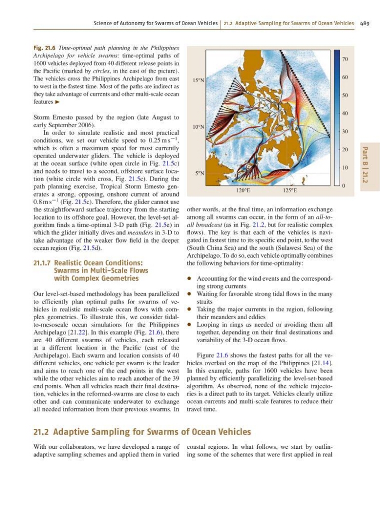
Fig. 21.6 Time-optimal path planning in the Philippines
Archipelago for vehicle swarms: time-optimal paths of
1600 vehicles deployed from 40 different release points in
the Pacific (marked by circles, in the east of the picture).
The vehicles cross the Philippines Archipelago from east
to west in the fastest time. Most of the paths are indirect as
they take advantage of currents and other multi-scale ocean
features I
Storm Ernesto passed by the region (late August to
early September 2006).
In order to simulate realistic and most practical
conditions, we set our vehicle speed to 0:25 m s
1 ,
which is often a maximum speed for most currently
operated underwater gliders. The vehicle is deployed
at the ocean surface (white open circle in Fig. 21.5c)
and needs to travel to a second, offshore surface location (white circle with cross, Fig. 21.5c). During the
path planning exercise, Tropical Storm Ernesto generates a strong, opposing, onshore current of around
0:8 m s
1 (Fig. 21.5c). Therefore, the glider cannot use
the straightforward surface trajectory from the starting
location to its offshore goal. However, the level-set algorithm finds a time-optimal 3-D path (Fig. 21.5e) in
which the glider initially dives and meanders in 3-D to
take advantage of the weaker flow field in the deeper
ocean region (Fig. 21.5d).
21.1.7 Realistic Ocean Conditions:
Swarms in Multi-Scale Flows
with Complex Geometries
Our level-set-based methodology has been parallelized
to efficiently plan optimal paths for swarms of vehicles in realistic multi-scale ocean flows with complex geometries. To illustrate this, we consider tidalto-mesoscale ocean simulations for the Philippines
Archipelago [21.22]. In this example (Fig. 21.6), there
are 40 different swarms of vehicles, each released
at a different location in the Pacific (east of the
Archipelago). Each swarm and location consists of 40
different vehicles, one vehicle per swarm is the leader
and aims to reach one of the end points in the west
while the other vehicles aim to reach another of the 39
end points. When all vehicles reach their final destination, vehicles in the reformed-swarms are close to each
other and can communicate underwater to exchange
all needed information from their previous swarms. In
120°E
125°E
15°N
10°N
5°N
70
60
50
40
30
20
10
0
other words, at the final time, an information exchange
among all swarms can occur, in the form of an all-toall broadcast (as in Fig. 21.2, but for realistic complex
flows). The key is that each of the vehicles is navigated in fastest time to its specific end point, to the west
(South China Sea) and the south (Sulawesi Sea) of the
Archipelago. To do so, each vehicle optimally combines
the following behaviors for time-optimality:
Accounting for the wind events and the corresponding strong currents
Waiting for favorable strong tidal flows in the many
straits
Taking the major currents in the region, following
their meanders and eddies
Looping in rings as needed or avoiding them all
together, depending on their final destinations and
variability of the 3-D ocean flows.
Figure 21.6 shows the fastest paths for all the vehicles overlaid on the map of the Philippines [21.14].
In this example, paths for 1600 vehicles have been
planned by efficiently parallelizing the level-set-based
algorithm. As observed, none of the vehicle trajectories is a direct path to its target. Vehicles clearly utilize
ocean currents and multi-scale features to reduce their
travel time.
21.2 Adaptive Sampling for Swarms of Ocean Vehicles
With our collaborators, we have developed a range of
adaptive sampling schemes and applied them in varied
coastal regions. In what follows, we start by outlining some of the schemes that were first applied in real
Part B | 21.2
Fig. 21.6 Time-optimal path planning in the Philippines
Archipelago for vehicle swarms: time-optimal paths of
1600 vehicles deployed from 40 different release points in
the Pacific (marked by circles, in the east of the picture).
The vehicles cross the Philippines Archipelago from east
to west in the fastest time. Most of the paths are indirect as
they take advantage of currents and other multi-scale ocean
features I
Storm Ernesto passed by the region (late August to
early September 2006).
In order to simulate realistic and most practical
conditions, we set our vehicle speed to 0:25 m s
1 ,
which is often a maximum speed for most currently
operated underwater gliders. The vehicle is deployed
at the ocean surface (white open circle in Fig. 21.5c)
and needs to travel to a second, offshore surface location (white circle with cross, Fig. 21.5c). During the
path planning exercise, Tropical Storm Ernesto generates a strong, opposing, onshore current of around
0:8 m s
1 (Fig. 21.5c). Therefore, the glider cannot use
the straightforward surface trajectory from the starting
location to its offshore goal. However, the level-set algorithm finds a time-optimal 3-D path (Fig. 21.5e) in
which the glider initially dives and meanders in 3-D to
take advantage of the weaker flow field in the deeper
ocean region (Fig. 21.5d).
21.1.7 Realistic Ocean Conditions:
Swarms in Multi-Scale Flows
with Complex Geometries
Our level-set-based methodology has been parallelized
to efficiently plan optimal paths for swarms of vehicles in realistic multi-scale ocean flows with complex geometries. To illustrate this, we consider tidalto-mesoscale ocean simulations for the Philippines
Archipelago [21.22]. In this example (Fig. 21.6), there
are 40 different swarms of vehicles, each released
at a different location in the Pacific (east of the
Archipelago). Each swarm and location consists of 40
different vehicles, one vehicle per swarm is the leader
and aims to reach one of the end points in the west
while the other vehicles aim to reach another of the 39
end points. When all vehicles reach their final destination, vehicles in the reformed-swarms are close to each
other and can communicate underwater to exchange
all needed information from their previous swarms. In
120°E
125°E
15°N
10°N
5°N
70
60
50
40
30
20
10
0
other words, at the final time, an information exchange
among all swarms can occur, in the form of an all-toall broadcast (as in Fig. 21.2, but for realistic complex
flows). The key is that each of the vehicles is navigated in fastest time to its specific end point, to the west
(South China Sea) and the south (Sulawesi Sea) of the
Archipelago. To do so, each vehicle optimally combines
the following behaviors for time-optimality:
Accounting for the wind events and the corresponding strong currents
Waiting for favorable strong tidal flows in the many
straits
Taking the major currents in the region, following
their meanders and eddies
Looping in rings as needed or avoiding them all
together, depending on their final destinations and
variability of the 3-D ocean flows.
Figure 21.6 shows the fastest paths for all the vehicles overlaid on the map of the Philippines [21.14].
In this example, paths for 1600 vehicles have been
planned by efficiently parallelizing the level-set-based
algorithm. As observed, none of the vehicle trajectories is a direct path to its target. Vehicles clearly utilize
ocean currents and multi-scale features to reduce their
travel time.
21.2 Adaptive Sampling for Swarms of Ocean Vehicles
With our collaborators, we have developed a range of
adaptive sampling schemes and applied them in varied
coastal regions. In what follows, we start by outlining some of the schemes that were first applied in real