

Science of Autonomy for Swarms of Ocean Vehicles 21.1 Time-Optimal Path Planning for Swarms of Ocean Vehicles 487
Part B | 21.1
Northern paths
Southern paths
0.2
0
0.4
Time = 0.029, u = [0.007, 17]
Time = 0.029, u = [0.007, 17]
y
x
y
x
0.6
0.8
1
a)
1
2
3
4
5
6
7
8
c) Travel time
Average uncertainty in path – standard devition
0.22
0.21
0.2
0.19
0.18
0.17
0.16
0.15
1
0.9
0.8
0.7
0.6
0.5
0.4
0.3
0.2
0.1
0
0.2
0
0.4
0.6
0.8
1
b) 1
0.9
0.8
0.7
0.6
0.5
0.4
0.3
0.2
0.1
0
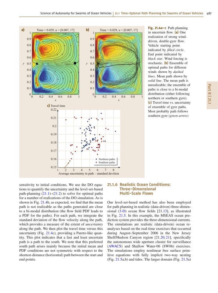
Fig. 21.4a–c Path planning
in uncertain flow. (a) One
realization of strong winddriven, double-gyre flow.
Vehicle starting point
indicated by filled circle.
End point indicated by
black star. Wind forcing is
stochastic. (b) Ensemble of
optimal paths for different
winds shown by dashed
lines. Mean path shown by
solid line. The mean path is
unrealizable; the ensemble of
paths is close to a bi-modal
distribution (either following
northern or southern gyre).
(c) Travel time vs. uncertainty
of ensemble of gyre paths.
Most probably path follows
southern gyre (green arrow)
sensitivity to initial conditions. We use the DO equations to quantify the uncertainty and the level-set-based
path-planning (21.1)–(21.2) to solve for optimal paths
for a number of realizations of the DO simulation. As is
shown in Fig. 21.4b, as expected, we find that the mean
path is not realizable as the paths generated are close
to a bi-modal distribution (the flow field PDF leads to
a PDF for the paths). For each path, we integrate the
standard deviation of the flow velocity along the path,
which provides a measure of the extent of uncertainty
along the path. We then plot the travel time versus this
uncertainty (Fig. 21.4c), providing a Pareto-like quantity. This plot indicates that a fast and least uncertain
path is a path to the south. We note that this preferred
south path arises mainly because the initial mean and
PDF conditions are not symmetric with respect to the
shortest-distance (horizontal) path between the start and
end points.
21.1.6 Realistic Ocean Conditions:
Three-Dimensional
Multi-Scale Flows
Our level-set-based method has also been employed
for path planning in realistic (data-driven) three-dimensional (3-D) ocean flow fields [21.13], as illustrated
in Fig. 21.5. In this example, the MSEAS ocean prediction system provides the three-dimensional currents.
The simulations are realistic (data-driven) ocean reanalyses based on the real-time exercises that occurred
during August–September 2006 in the New Jersey
Shelf/Hudson Canyon region [21.20, 21], specifically
the autonomous wide aperture cluster for surveillance
(AWACS) and Shallow Water-06 (SW06) exercises.
The simulations employ nonlinear free surface primitive equations with fully implicit two-way nesting
(Fig. 21.5a,b) and tides. The larger domain (Fig. 21.5a)
Part B | 21.1
Northern paths
Southern paths
0.2
0
0.4
Time = 0.029, u = [0.007, 17]
Time = 0.029, u = [0.007, 17]
y
x
y
x
0.6
0.8
1
a)
1
2
3
4
5
6
7
8
c) Travel time
Average uncertainty in path – standard devition
0.22
0.21
0.2
0.19
0.18
0.17
0.16
0.15
1
0.9
0.8
0.7
0.6
0.5
0.4
0.3
0.2
0.1
0
0.2
0
0.4
0.6
0.8
1
b) 1
0.9
0.8
0.7
0.6
0.5
0.4
0.3
0.2
0.1
0
Fig. 21.4a–c Path planning
in uncertain flow. (a) One
realization of strong winddriven, double-gyre flow.
Vehicle starting point
indicated by filled circle.
End point indicated by
black star. Wind forcing is
stochastic. (b) Ensemble of
optimal paths for different
winds shown by dashed
lines. Mean path shown by
solid line. The mean path is
unrealizable; the ensemble of
paths is close to a bi-modal
distribution (either following
northern or southern gyre).
(c) Travel time vs. uncertainty
of ensemble of gyre paths.
Most probably path follows
southern gyre (green arrow)
sensitivity to initial conditions. We use the DO equations to quantify the uncertainty and the level-set-based
path-planning (21.1)–(21.2) to solve for optimal paths
for a number of realizations of the DO simulation. As is
shown in Fig. 21.4b, as expected, we find that the mean
path is not realizable as the paths generated are close
to a bi-modal distribution (the flow field PDF leads to
a PDF for the paths). For each path, we integrate the
standard deviation of the flow velocity along the path,
which provides a measure of the extent of uncertainty
along the path. We then plot the travel time versus this
uncertainty (Fig. 21.4c), providing a Pareto-like quantity. This plot indicates that a fast and least uncertain
path is a path to the south. We note that this preferred
south path arises mainly because the initial mean and
PDF conditions are not symmetric with respect to the
shortest-distance (horizontal) path between the start and
end points.
21.1.6 Realistic Ocean Conditions:
Three-Dimensional
Multi-Scale Flows
Our level-set-based method has also been employed
for path planning in realistic (data-driven) three-dimensional (3-D) ocean flow fields [21.13], as illustrated
in Fig. 21.5. In this example, the MSEAS ocean prediction system provides the three-dimensional currents.
The simulations are realistic (data-driven) ocean reanalyses based on the real-time exercises that occurred
during August–September 2006 in the New Jersey
Shelf/Hudson Canyon region [21.20, 21], specifically
the autonomous wide aperture cluster for surveillance
(AWACS) and Shallow Water-06 (SW06) exercises.
The simulations employ nonlinear free surface primitive equations with fully implicit two-way nesting
(Fig. 21.5a,b) and tides. The larger domain (Fig. 21.5a)