

Part B | 21.1
486 Part B Autonomous Ocean Vehicles, Subsystems and Control
0
2
6
7
1
3
4
5
a)
1
0.8
0.6
0.4
0.2
0
0
2
6
7
1
3
4
5
c)
1
0.8
0.6
0.4
0.2
0
0
2
6
7
1
3
4
5
d)
1
0.8
0.6
0.4
0.2
0
2.5
2
1.5
1
0.5
0
0
2
6
7
1
3
4
5
b)
1
0.8
0.6
0.4
0.2
0
2.5
2
1.5
1
0.5
0
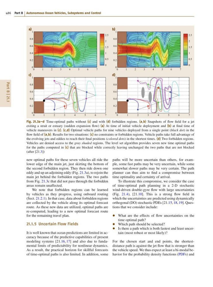
Fig. 21.3a–d Time-optimal paths without (c) and with (d) forbidden regions. (a,b) Snapshots of flow field for a jet
exiting a strait or estuary (sudden expansion flow) (a) At time of initial vehicle deployment and (b) at final time of
vehicle maneuvers in (c). (c,d) Optimal vehicle paths for nine vehicles deployed from a single point (black dot) in the
flow field of (a,b). Results for two situations: (c) no constraints or forbidden regions. Vehicle paths take full advantage of
the evolving jets and eddies to reach their final positions (colored dots) in the shortest times. (d) Two forbidden regions.
Vehicles are denied access to the gray shaded regions. The level set algorithm provides seven new time optimal paths
for the paths computed in (c) that are blocked while correctly leaving unchanged the two paths that are not blocked
(after [21.3])
new optimal paths for these seven vehicles all ride the
lower edge of the main jet, just skirting the bottom of
the second forbidden region. They then ride down one
eddy and up an adjoining eddy (Fig. 21.3a), to rejoin the
main jet behind the forbidden regions. The two paths
from Fig. 21.3c that did not pass through the forbidden
areas remain unaffected.
We note that forbidden regions can be learned
by vehicles as they progress, using onboard routing
(Sect. 21.2.1). In that case, data about forbidden regions
are collected by the vehicle along its optimal forecast
route. As these new data are utilized, optimal paths are
re-computed, leading to a new optimal forecast route
for the remaining travel plan.
21.1.5 Uncertain Flow Fields
It is well known that ocean predictions are limited in accuracy because of the predictive capabilities of present
modeling systems [21.16, 17] and also due to fundamental limits of predictability for nonlinear dynamics.
As a result, the practical horizon for skillful forecasts
of time-optimal paths is also limited. In addition, some
paths will be more uncertain than others, for example, some fast paths may be very uncertain, while some
somewhat slower paths may be very certain. The path
planner can thus aim to find a compromise between
time optimality and certainty of arrival.
To illustrate this compromise, we consider the case
of time-optimal path planning in a 2-D stochastic
wind-driven double-gyre flow with large uncertainties
(Fig. 21.4), [21.10]. This is a strong flow field in
which the uncertainties are predicted using dynamically
orthogonal (DO) stochastic PDEs [21.15, 18, 19]. Questions that we consider include:
What are the effects of flow uncertainties on the
time optimal path?
Which path should be selected?
Is there a path which is both fastest and least uncertain (most robust or most likely)?
For the chosen start and end points, the shortestdistance path is against the jet flow that is stronger than
the vehicle speed. We thus expect at least a bi-modal behavior for the probability density functions (PDFs) and
486 Part B Autonomous Ocean Vehicles, Subsystems and Control
0
2
6
7
1
3
4
5
a)
1
0.8
0.6
0.4
0.2
0
0
2
6
7
1
3
4
5
c)
1
0.8
0.6
0.4
0.2
0
0
2
6
7
1
3
4
5
d)
1
0.8
0.6
0.4
0.2
0
2.5
2
1.5
1
0.5
0
0
2
6
7
1
3
4
5
b)
1
0.8
0.6
0.4
0.2
0
2.5
2
1.5
1
0.5
0
Fig. 21.3a–d Time-optimal paths without (c) and with (d) forbidden regions. (a,b) Snapshots of flow field for a jet
exiting a strait or estuary (sudden expansion flow) (a) At time of initial vehicle deployment and (b) at final time of
vehicle maneuvers in (c). (c,d) Optimal vehicle paths for nine vehicles deployed from a single point (black dot) in the
flow field of (a,b). Results for two situations: (c) no constraints or forbidden regions. Vehicle paths take full advantage of
the evolving jets and eddies to reach their final positions (colored dots) in the shortest times. (d) Two forbidden regions.
Vehicles are denied access to the gray shaded regions. The level set algorithm provides seven new time optimal paths
for the paths computed in (c) that are blocked while correctly leaving unchanged the two paths that are not blocked
(after [21.3])
new optimal paths for these seven vehicles all ride the
lower edge of the main jet, just skirting the bottom of
the second forbidden region. They then ride down one
eddy and up an adjoining eddy (Fig. 21.3a), to rejoin the
main jet behind the forbidden regions. The two paths
from Fig. 21.3c that did not pass through the forbidden
areas remain unaffected.
We note that forbidden regions can be learned
by vehicles as they progress, using onboard routing
(Sect. 21.2.1). In that case, data about forbidden regions
are collected by the vehicle along its optimal forecast
route. As these new data are utilized, optimal paths are
re-computed, leading to a new optimal forecast route
for the remaining travel plan.
21.1.5 Uncertain Flow Fields
It is well known that ocean predictions are limited in accuracy because of the predictive capabilities of present
modeling systems [21.16, 17] and also due to fundamental limits of predictability for nonlinear dynamics.
As a result, the practical horizon for skillful forecasts
of time-optimal paths is also limited. In addition, some
paths will be more uncertain than others, for example, some fast paths may be very uncertain, while some
somewhat slower paths may be very certain. The path
planner can thus aim to find a compromise between
time optimality and certainty of arrival.
To illustrate this compromise, we consider the case
of time-optimal path planning in a 2-D stochastic
wind-driven double-gyre flow with large uncertainties
(Fig. 21.4), [21.10]. This is a strong flow field in
which the uncertainties are predicted using dynamically
orthogonal (DO) stochastic PDEs [21.15, 18, 19]. Questions that we consider include:
What are the effects of flow uncertainties on the
time optimal path?
Which path should be selected?
Is there a path which is both fastest and least uncertain (most robust or most likely)?
For the chosen start and end points, the shortestdistance path is against the jet flow that is stronger than
the vehicle speed. We thus expect at least a bi-modal behavior for the probability density functions (PDFs) and