

Part B | 20.6
472 Part B Autonomous Ocean Vehicles, Subsystems and Control
0
2000
4000
Temperature variation with depth and time
6000
8000
a) z (m)
Time since mission start (s)
0
–5
–10
–15
–20
–25
–30
–35
10
9
1 2
11
15
13
Temperature-depth profile
14
16
b) z (m)
Temperature (°C)
0
–5
–10
–15
–20
–25
–30
–35
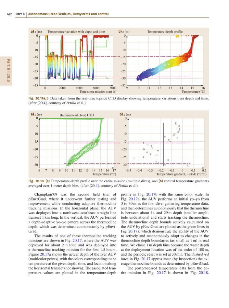
Fig. 20.17a,b Data taken from the real-time topside CTD display showing temperature variations over depth and time.
(after [20.4], courtesy of Petillo et al.)
7
8
6
1 0 1 1
9
1 3
1 5 1 6
12
Hammerhead (Iver) CTD
14
17
a) z (m)
Temperature (°C)
0
–5
–10
–15
–20
–25
–30
0
–5
–10
–15
–20
–25
–30
–0.4
–0.5
–0.2
–0.3
0.1
–0.1
0
0.2
b) z (m)
Temperature gradient, – dT/dz (°C/m)
Fig. 20.18 (a) Temperature-depth profile over the entire mission (multiple dives), and (b) vertical temperature gradients
averaged over 1-meter depth bins. (after [20.4], courtesy of Petillo et al.)
Champlain’09 was the second field trial of
pEnvtGrad, where it underwent further testing and
improvement while conducting adaptive thermocline
tracking missions. In the horizontal plane, the AUV
was deployed into a northwest–southeast straight line
transect 1 km long. In the vertical, the AUV performed
a depth-adaptive yo–yo pattern across the thermocline
depth, which was determined autonomously by pEnvtGrad.
The results of one of these thermocline tracking
missions are shown in Fig. 20.17, where the AUV was
deployed for about 2 h total and was deployed into
a thermocline tracking mission for the first 1.5 hours.
Figure 20.17a shows the actual depth of the Iver AUV
(multicolor points), with the colors corresponding to the
temperature at the given depth, time, and location along
the horizontal transect (not shown). The associated temperature values are plotted in the temperature-depth
profile in Fig. 20.17b with the same color scale. In
Fig. 20.17a, the AUV performs an initial yo–yo from
3 to 30 m as the first dive, gathering temperature data,
and then determines autonomously that the thermocline
is between about 14 and 29 m depth (smaller amplitude undulations) and starts tracking the thermocline.
The thermocline depth bounds actively calculated on
the AUV by pEnvtGrad are plotted as the green lines in
Fig. 20.17a, which demonstrate the ability of the AUV
to actively and autonomously adapt to changes in the
thermocline depth boundaries (as small as 1 m) in real
time. We chose 1 m depth bins because the water depth
at the deployment location was of the order of 100 m,
and the periodic reset was set at 30 min. The dashed red
lines in Fig. 20.17 approximate (by inspection) the average thermocline bounds as determined by pEnvtGrad.
The postprocessed temperature data from the entire mission in Fig. 20.17 is shown in Fig. 20.18.
472 Part B Autonomous Ocean Vehicles, Subsystems and Control
0
2000
4000
Temperature variation with depth and time
6000
8000
a) z (m)
Time since mission start (s)
0
–5
–10
–15
–20
–25
–30
–35
10
9
1 2
11
15
13
Temperature-depth profile
14
16
b) z (m)
Temperature (°C)
0
–5
–10
–15
–20
–25
–30
–35
Fig. 20.17a,b Data taken from the real-time topside CTD display showing temperature variations over depth and time.
(after [20.4], courtesy of Petillo et al.)
7
8
6
1 0 1 1
9
1 3
1 5 1 6
12
Hammerhead (Iver) CTD
14
17
a) z (m)
Temperature (°C)
0
–5
–10
–15
–20
–25
–30
0
–5
–10
–15
–20
–25
–30
–0.4
–0.5
–0.2
–0.3
0.1
–0.1
0
0.2
b) z (m)
Temperature gradient, – dT/dz (°C/m)
Fig. 20.18 (a) Temperature-depth profile over the entire mission (multiple dives), and (b) vertical temperature gradients
averaged over 1-meter depth bins. (after [20.4], courtesy of Petillo et al.)
Champlain’09 was the second field trial of
pEnvtGrad, where it underwent further testing and
improvement while conducting adaptive thermocline
tracking missions. In the horizontal plane, the AUV
was deployed into a northwest–southeast straight line
transect 1 km long. In the vertical, the AUV performed
a depth-adaptive yo–yo pattern across the thermocline
depth, which was determined autonomously by pEnvtGrad.
The results of one of these thermocline tracking
missions are shown in Fig. 20.17, where the AUV was
deployed for about 2 h total and was deployed into
a thermocline tracking mission for the first 1.5 hours.
Figure 20.17a shows the actual depth of the Iver AUV
(multicolor points), with the colors corresponding to the
temperature at the given depth, time, and location along
the horizontal transect (not shown). The associated temperature values are plotted in the temperature-depth
profile in Fig. 20.17b with the same color scale. In
Fig. 20.17a, the AUV performs an initial yo–yo from
3 to 30 m as the first dive, gathering temperature data,
and then determines autonomously that the thermocline
is between about 14 and 29 m depth (smaller amplitude undulations) and starts tracking the thermocline.
The thermocline depth bounds actively calculated on
the AUV by pEnvtGrad are plotted as the green lines in
Fig. 20.17a, which demonstrate the ability of the AUV
to actively and autonomously adapt to changes in the
thermocline depth boundaries (as small as 1 m) in real
time. We chose 1 m depth bins because the water depth
at the deployment location was of the order of 100 m,
and the periodic reset was set at 30 min. The dashed red
lines in Fig. 20.17 approximate (by inspection) the average thermocline bounds as determined by pEnvtGrad.
The postprocessed temperature data from the entire mission in Fig. 20.17 is shown in Fig. 20.18.