

Nested Autonomy for Distributed Ocean Sensing 20.6 Application Examples 471
Part B | 20.6
1500 1510 1520
OEX CTD – sound speed
1530 1540
a) z (m)
Sound speed (m/s)
0
–10
–20
–30
–40
–50
–60
–5
0
5
Sound speed gradient
–dc/dz ((m/s)/m)
0
–10
–20
–30
–40
–50
–60
10
15
20
OEX CTD – temperature
25
b) z (m)
Temperature (°C)
0
–10
–20
–30
–40
–50
–60
–2
–1
0
1
Temperature gradient
–dT/dz (°C/m)
0
–10
–20
–30
–40
–50
–60
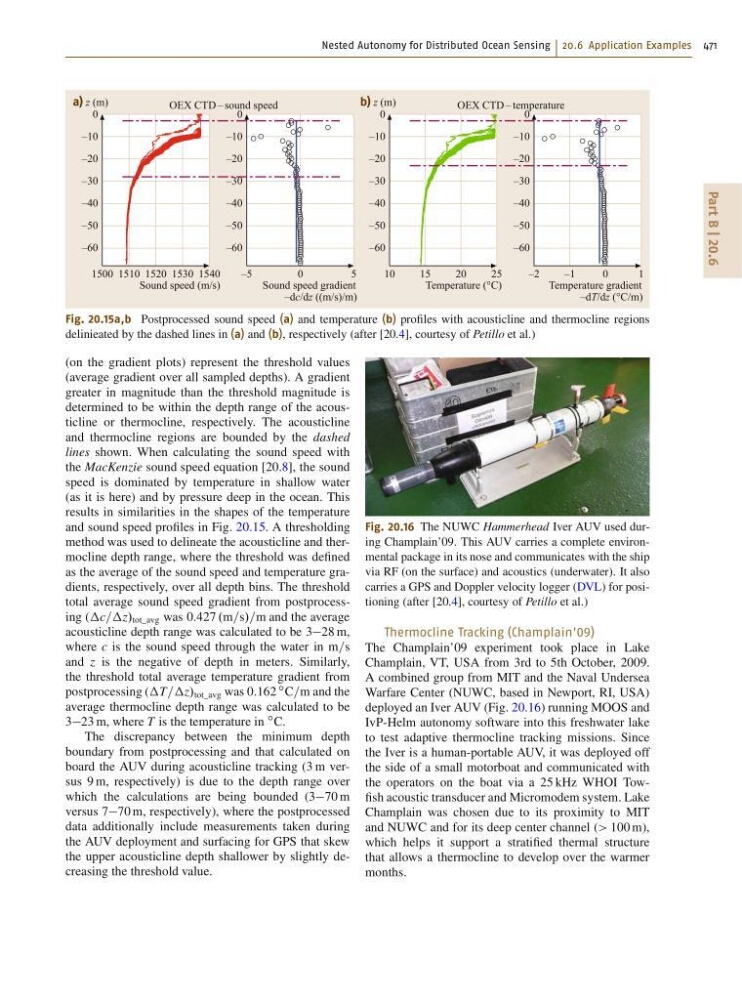
Fig. 20.15a,b Postprocessed sound speed (a) and temperature (b) profiles with acousticline and thermocline regions
delinieated by the dashed lines in (a) and (b), respectively (after [20.4], courtesy of Petillo et al.)
(on the gradient plots) represent the threshold values
(average gradient over all sampled depths). A gradient
greater in magnitude than the threshold magnitude is
determined to be within the depth range of the acousticline or thermocline, respectively. The acousticline
and thermocline regions are bounded by the dashed
lines shown. When calculating the sound speed with
the MacKenzie sound speed equation [20.8], the sound
speed is dominated by temperature in shallow water
(as it is here) and by pressure deep in the ocean. This
results in similarities in the shapes of the temperature
and sound speed profiles in Fig. 20.15. A thresholding
method was used to delineate the acousticline and thermocline depth range, where the threshold was defined
as the average of the sound speed and temperature gradients, respectively, over all depth bins. The threshold
total average sound speed gradient from postprocessing (c=z/ tot_avg was 0:427 .m=s/=m and the average
acousticline depth range was calculated to be 328 m,
where c is the sound speed through the water in m=s
and z is the negative of depth in meters. Similarly,
the threshold total average temperature gradient from
postprocessing (T=z/ tot_avg was 0:162
ı C=m and the
average thermocline depth range was calculated to be
323 m, where T is the temperature in
ı C.
The discrepancy between the minimum depth
boundary from postprocessing and that calculated on
board the AUV during acousticline tracking (3 m versus 9 m, respectively) is due to the depth range over
which the calculations are being bounded (370 m
versus 770 m, respectively), where the postprocessed
data additionally include measurements taken during
the AUV deployment and surfacing for GPS that skew
the upper acousticline depth shallower by slightly decreasing the threshold value.
Fig. 20.16 The NUWC Hammerhead Iver AUV used during Champlain’09. This AUV carries a complete environmental package in its nose and communicates with the ship
via RF (on the surface) and acoustics (underwater). It also
carries a GPS and Doppler velocity logger (DVL) for positioning (after [20.4], courtesy of Petillo et al.)
Thermocline Tracking (Champlain’09)
The Champlain’09 experiment took place in Lake
Champlain, VT, USA from 3rd to 5th October, 2009.
A combined group from MIT and the Naval Undersea
Warfare Center (NUWC, based in Newport, RI, USA)
deployed an Iver AUV (Fig. 20.16) running MOOS and
IvP-Helm autonomy software into this freshwater lake
to test adaptive thermocline tracking missions. Since
the Iver is a human-portable AUV, it was deployed off
the side of a small motorboat and communicated with
the operators on the boat via a 25 kHz WHOI Towfish acoustic transducer and Micromodem system. Lake
Champlain was chosen due to its proximity to MIT
and NUWC and for its deep center channel (> 100 m),
which helps it support a stratified thermal structure
that allows a thermocline to develop over the warmer
months.
Part B | 20.6
1500 1510 1520
OEX CTD – sound speed
1530 1540
a) z (m)
Sound speed (m/s)
0
–10
–20
–30
–40
–50
–60
–5
0
5
Sound speed gradient
–dc/dz ((m/s)/m)
0
–10
–20
–30
–40
–50
–60
10
15
20
OEX CTD – temperature
25
b) z (m)
Temperature (°C)
0
–10
–20
–30
–40
–50
–60
–2
–1
0
1
Temperature gradient
–dT/dz (°C/m)
0
–10
–20
–30
–40
–50
–60
Fig. 20.15a,b Postprocessed sound speed (a) and temperature (b) profiles with acousticline and thermocline regions
delinieated by the dashed lines in (a) and (b), respectively (after [20.4], courtesy of Petillo et al.)
(on the gradient plots) represent the threshold values
(average gradient over all sampled depths). A gradient
greater in magnitude than the threshold magnitude is
determined to be within the depth range of the acousticline or thermocline, respectively. The acousticline
and thermocline regions are bounded by the dashed
lines shown. When calculating the sound speed with
the MacKenzie sound speed equation [20.8], the sound
speed is dominated by temperature in shallow water
(as it is here) and by pressure deep in the ocean. This
results in similarities in the shapes of the temperature
and sound speed profiles in Fig. 20.15. A thresholding
method was used to delineate the acousticline and thermocline depth range, where the threshold was defined
as the average of the sound speed and temperature gradients, respectively, over all depth bins. The threshold
total average sound speed gradient from postprocessing (c=z/ tot_avg was 0:427 .m=s/=m and the average
acousticline depth range was calculated to be 328 m,
where c is the sound speed through the water in m=s
and z is the negative of depth in meters. Similarly,
the threshold total average temperature gradient from
postprocessing (T=z/ tot_avg was 0:162
ı C=m and the
average thermocline depth range was calculated to be
323 m, where T is the temperature in
ı C.
The discrepancy between the minimum depth
boundary from postprocessing and that calculated on
board the AUV during acousticline tracking (3 m versus 9 m, respectively) is due to the depth range over
which the calculations are being bounded (370 m
versus 770 m, respectively), where the postprocessed
data additionally include measurements taken during
the AUV deployment and surfacing for GPS that skew
the upper acousticline depth shallower by slightly decreasing the threshold value.
Fig. 20.16 The NUWC Hammerhead Iver AUV used during Champlain’09. This AUV carries a complete environmental package in its nose and communicates with the ship
via RF (on the surface) and acoustics (underwater). It also
carries a GPS and Doppler velocity logger (DVL) for positioning (after [20.4], courtesy of Petillo et al.)
Thermocline Tracking (Champlain’09)
The Champlain’09 experiment took place in Lake
Champlain, VT, USA from 3rd to 5th October, 2009.
A combined group from MIT and the Naval Undersea
Warfare Center (NUWC, based in Newport, RI, USA)
deployed an Iver AUV (Fig. 20.16) running MOOS and
IvP-Helm autonomy software into this freshwater lake
to test adaptive thermocline tracking missions. Since
the Iver is a human-portable AUV, it was deployed off
the side of a small motorboat and communicated with
the operators on the boat via a 25 kHz WHOI Towfish acoustic transducer and Micromodem system. Lake
Champlain was chosen due to its proximity to MIT
and NUWC and for its deep center channel (> 100 m),
which helps it support a stratified thermal structure
that allows a thermocline to develop over the warmer
months.