

Acoustic Communication 15.4 Propagation Channel 367
Part B | 15.4
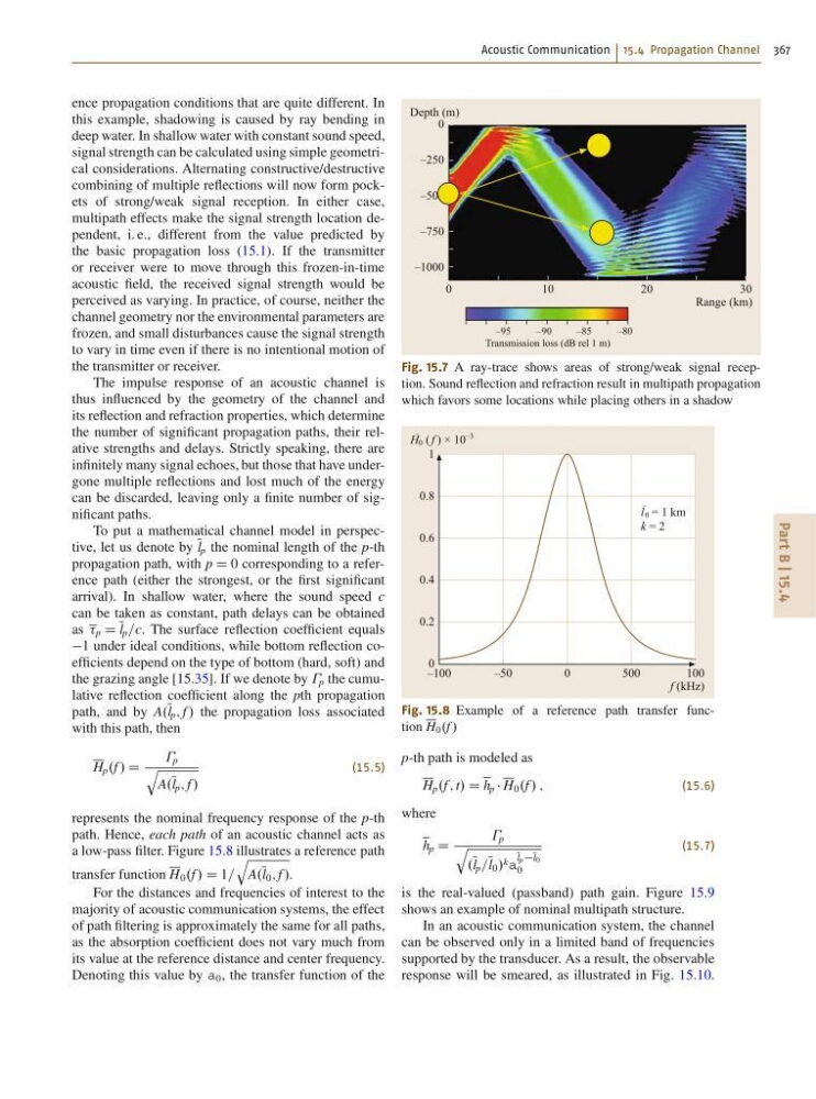
ence propagation conditions that are quite different. In
this example, shadowing is caused by ray bending in
deep water. In shallow water with constant sound speed,
signal strength can be calculated using simple geometrical considerations. Alternating constructive/destructive
combining of multiple reflections will now form pockets of strong/weak signal reception. In either case,
multipath effects make the signal strength location dependent, i. e., different from the value predicted by
the basic propagation loss (15.1). If the transmitter
or receiver were to move through this frozen-in-time
acoustic field, the received signal strength would be
perceived as varying. In practice, of course, neither the
channel geometry nor the environmental parameters are
frozen, and small disturbances cause the signal strength
to vary in time even if there is no intentional motion of
the transmitter or receiver.
The impulse response of an acoustic channel is
thus influenced by the geometry of the channel and
its reflection and refraction properties, which determine
the number of significant propagation paths, their relative strengths and delays. Strictly speaking, there are
infinitely many signal echoes, but those that have undergone multiple reflections and lost much of the energy
can be discarded, leaving only a finite number of significant paths.
To put a mathematical channel model in perspective, let us denote by l p the nominal length of the p-th
propagation path, with p D 0 corresponding to a reference path (either the strongest, or the first significant
arrival). In shallow water, where the sound speed c
can be taken as constant, path delays can be obtained
as p D l p =c. The surface reflection coefficient equals
1 under ideal conditions, while bottom reflection coefficients depend on the type of bottom (hard, soft) and
the grazing angle [15.35]. If we denote by p the cumulative reflection coefficient along the pth propagation
path, and by A.l p ; f / the propagation loss associated
with this path, then
H p .f / D
p
q
A.l p ; f /
(15.5)
represents the nominal frequency response of the p-th
path. Hence, each path of an acoustic channel acts as
a low-pass filter. Figure 15.8 illustrates a reference path
transfer function H 0 .f / D 1=
q
A.l 0 ; f /.
For the distances and frequencies of interest to the
majority of acoustic communication systems, the effect
of path filtering is approximately the same for all paths,
as the absorption coefficient does not vary much from
its value at the reference distance and center frequency.
Denoting this value by a 0 , the transfer function of the
0
1 0
–95
–90
–85
–80
20
30
Depth (m)
Range (km)
Transmission loss (dB rel 1 m)
0
–250
–500
–750
–1000
Fig. 15.7 A ray-trace shows areas of strong/weak signal reception. Sound reflection and refraction result in multipath propagation
which favors some locations while placing others in a shadow
–100
–50
0
l
–
0 = 1 km
k = 2
500
100
H
–
0 ( f ) × 10
–3
f (kHz)
1
0.8
0.6
0.4
0.2
0
Fig. 15.8 Example of a reference path transfer function H 0 .f /
p-th path is modeled as
H p .f ; t/ D h p H 0 .f / ;
(15.6)
where
h p D
p
q
.l p =l 0 / k a
lpl0
0
(15.7)
is the real-valued (passband) path gain. Figure 15.9
shows an example of nominal multipath structure.
In an acoustic communication system, the channel
can be observed only in a limited band of frequencies
supported by the transducer. As a result, the observable
response will be smeared, as illustrated in Fig. 15.10.
Part B | 15.4
ence propagation conditions that are quite different. In
this example, shadowing is caused by ray bending in
deep water. In shallow water with constant sound speed,
signal strength can be calculated using simple geometrical considerations. Alternating constructive/destructive
combining of multiple reflections will now form pockets of strong/weak signal reception. In either case,
multipath effects make the signal strength location dependent, i. e., different from the value predicted by
the basic propagation loss (15.1). If the transmitter
or receiver were to move through this frozen-in-time
acoustic field, the received signal strength would be
perceived as varying. In practice, of course, neither the
channel geometry nor the environmental parameters are
frozen, and small disturbances cause the signal strength
to vary in time even if there is no intentional motion of
the transmitter or receiver.
The impulse response of an acoustic channel is
thus influenced by the geometry of the channel and
its reflection and refraction properties, which determine
the number of significant propagation paths, their relative strengths and delays. Strictly speaking, there are
infinitely many signal echoes, but those that have undergone multiple reflections and lost much of the energy
can be discarded, leaving only a finite number of significant paths.
To put a mathematical channel model in perspective, let us denote by l p the nominal length of the p-th
propagation path, with p D 0 corresponding to a reference path (either the strongest, or the first significant
arrival). In shallow water, where the sound speed c
can be taken as constant, path delays can be obtained
as p D l p =c. The surface reflection coefficient equals
1 under ideal conditions, while bottom reflection coefficients depend on the type of bottom (hard, soft) and
the grazing angle [15.35]. If we denote by p the cumulative reflection coefficient along the pth propagation
path, and by A.l p ; f / the propagation loss associated
with this path, then
H p .f / D
p
q
A.l p ; f /
(15.5)
represents the nominal frequency response of the p-th
path. Hence, each path of an acoustic channel acts as
a low-pass filter. Figure 15.8 illustrates a reference path
transfer function H 0 .f / D 1=
q
A.l 0 ; f /.
For the distances and frequencies of interest to the
majority of acoustic communication systems, the effect
of path filtering is approximately the same for all paths,
as the absorption coefficient does not vary much from
its value at the reference distance and center frequency.
Denoting this value by a 0 , the transfer function of the
0
1 0
–95
–90
–85
–80
20
30
Depth (m)
Range (km)
Transmission loss (dB rel 1 m)
0
–250
–500
–750
–1000
Fig. 15.7 A ray-trace shows areas of strong/weak signal reception. Sound reflection and refraction result in multipath propagation
which favors some locations while placing others in a shadow
–100
–50
0
l
–
0 = 1 km
k = 2
500
100
H
–
0 ( f ) × 10
–3
f (kHz)
1
0.8
0.6
0.4
0.2
0
Fig. 15.8 Example of a reference path transfer function H 0 .f /
p-th path is modeled as
H p .f ; t/ D h p H 0 .f / ;
(15.6)
where
h p D
p
q
.l p =l 0 / k a
lpl0
0
(15.7)
is the real-valued (passband) path gain. Figure 15.9
shows an example of nominal multipath structure.
In an acoustic communication system, the channel
can be observed only in a limited band of frequencies
supported by the transducer. As a result, the observable
response will be smeared, as illustrated in Fig. 15.10.