

Part B | 15.4
364 Part B Autonomous Ocean Vehicles, Subsystems and Control
tial location, and frequency. The accurate representation
of such a complex and dynamic system at any time, location, and frequency is simply not possible. As a result,
even the most sophisticated models often display significant difference with measurements. Significant efforts
are made to adapt the statistical models developed for
radio communications, but much work remains in making these models sufficiently accurate.
Various scientific and governmental organizations
(spearheaded by the United States Office of Naval Research), have developed series of comparative tests for
existing technology and signal waveforms (Signal-ex,
Modem-ex, KAM’11 [15.27]) and underwater acoustic networks (e.g., SeaWeb [15.28]). One key benefit of
such tests is the careful monitoring of environmental
characteristics during the test.
15.4 Propagation Channel
15.4.1 Attenuation and Noise
A distinguishing property of acoustic channels is the
fact that the path loss depends on the signal frequency.
This dependence is a consequence of absorption, i. e.,
transfer of acoustic energy into heat. In addition to
the absorption loss, signal experiences a spreading loss
which increases with distance. The overall path loss is
given by [15.29]
A.l; f / D .l=l ref /
k a.f /
llref
;
(15.1)
where f is the signal frequency and l is the transmission
distance, taken in reference to some l ref . The path loss
exponent k models the spreading loss, and its usual values are between 1 and 2, for cylindrical and spherical
spreading, respectively. The absorption coefficient can
be expressed empirically, using Thorp’s formula, which
gives a.f / in dB=km for f in kHz as [15.29]
10 log a.f / D 0:11
f
2
1 C f 2 C 44
f
2
4100 C f 2
C 2:75 10
4 f
2
C 0:003 :
(15.2)
This formula is generally valid for frequencies above
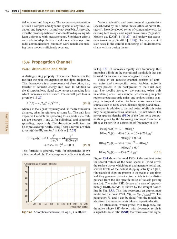
a few hundred Hz. The absorption coefficient is shown
0 20 40 60 80 100 120 140
180
160
200
Absorption coefficient (dB/km)
Frequency (kHz)
60
50
40
30
20
10
0
Fig. 15.3 Absorption coefficient, 10 log a.f / in dB=km
in Fig. 15.3. It increases rapidly with frequency, thus
imposing a limit on the operational bandwidth that can
be used for an acoustic link of a given distance.
Noise in an acoustic channel consists of ambient noise and site-specific noise. Ambient noise is
always present in the background of the quiet deep
sea. Site-specific noise, on the contrary, exists only
in certain places. For example, ice cracking in polar
regions creates acoustic noise, and so does shrimp snapping in tropical waters. Ambient noise comes from
sources such as turbulence, distant shipping, and breaking waves, in addition to thermal noise. While this noise
may be approximated as Gaussian, it is not white. The
power spectral density (PSD) of the four noise components is given by the following empirical formulae in
dB re Pa per Hz as a function of frequency in kHz
10 log N t .f / D 17 30 log f
10 log N s .f / D 40 C 20.s 0:5/ C 26 log f
60 log.f C 0:03/
10 log N w .f / D 50 C 7:5w
1=2
C 20 log f
40 log.f C 0:4/
10 log N th .f / D D15 C 20 log f :
(15.3)
Figure 15.4 shows the total PSD of the ambient noise
for several values of the wind speed w (wind drives
the surface waves which break and generate noise) and
several levels of the distant shipping activity s 2 Œ0; 1
(thousands of ships are present in the ocean at any time,
and they generate distant noise, which is to be distinguished from the site-specific noise of vessels passing
nearby). The noise PSD decays at a rate of approximately 18 dB=decade, as shown by the straight dashed
line in Fig. 15.4. This line represents an approximate
model for the noise PSD, N.f / D N 0 .f =f refx /
Á . The
parameters N 0 and Á can be fitted from the model, but
also from the measurements taken at a particular site.
The attenuation, which grows with frequency, and
the noise whose PSD decays with frequency, result in
a signal-to-noise ratio (SNR) that varies over the signal
364 Part B Autonomous Ocean Vehicles, Subsystems and Control
tial location, and frequency. The accurate representation
of such a complex and dynamic system at any time, location, and frequency is simply not possible. As a result,
even the most sophisticated models often display significant difference with measurements. Significant efforts
are made to adapt the statistical models developed for
radio communications, but much work remains in making these models sufficiently accurate.
Various scientific and governmental organizations
(spearheaded by the United States Office of Naval Research), have developed series of comparative tests for
existing technology and signal waveforms (Signal-ex,
Modem-ex, KAM’11 [15.27]) and underwater acoustic networks (e.g., SeaWeb [15.28]). One key benefit of
such tests is the careful monitoring of environmental
characteristics during the test.
15.4 Propagation Channel
15.4.1 Attenuation and Noise
A distinguishing property of acoustic channels is the
fact that the path loss depends on the signal frequency.
This dependence is a consequence of absorption, i. e.,
transfer of acoustic energy into heat. In addition to
the absorption loss, signal experiences a spreading loss
which increases with distance. The overall path loss is
given by [15.29]
A.l; f / D .l=l ref /
k a.f /
llref
;
(15.1)
where f is the signal frequency and l is the transmission
distance, taken in reference to some l ref . The path loss
exponent k models the spreading loss, and its usual values are between 1 and 2, for cylindrical and spherical
spreading, respectively. The absorption coefficient can
be expressed empirically, using Thorp’s formula, which
gives a.f / in dB=km for f in kHz as [15.29]
10 log a.f / D 0:11
f
2
1 C f 2 C 44
f
2
4100 C f 2
C 2:75 10
4 f
2
C 0:003 :
(15.2)
This formula is generally valid for frequencies above
a few hundred Hz. The absorption coefficient is shown
0 20 40 60 80 100 120 140
180
160
200
Absorption coefficient (dB/km)
Frequency (kHz)
60
50
40
30
20
10
0
Fig. 15.3 Absorption coefficient, 10 log a.f / in dB=km
in Fig. 15.3. It increases rapidly with frequency, thus
imposing a limit on the operational bandwidth that can
be used for an acoustic link of a given distance.
Noise in an acoustic channel consists of ambient noise and site-specific noise. Ambient noise is
always present in the background of the quiet deep
sea. Site-specific noise, on the contrary, exists only
in certain places. For example, ice cracking in polar
regions creates acoustic noise, and so does shrimp snapping in tropical waters. Ambient noise comes from
sources such as turbulence, distant shipping, and breaking waves, in addition to thermal noise. While this noise
may be approximated as Gaussian, it is not white. The
power spectral density (PSD) of the four noise components is given by the following empirical formulae in
dB re Pa per Hz as a function of frequency in kHz
10 log N t .f / D 17 30 log f
10 log N s .f / D 40 C 20.s 0:5/ C 26 log f
60 log.f C 0:03/
10 log N w .f / D 50 C 7:5w
1=2
C 20 log f
40 log.f C 0:4/
10 log N th .f / D D15 C 20 log f :
(15.3)
Figure 15.4 shows the total PSD of the ambient noise
for several values of the wind speed w (wind drives
the surface waves which break and generate noise) and
several levels of the distant shipping activity s 2 Œ0; 1
(thousands of ships are present in the ocean at any time,
and they generate distant noise, which is to be distinguished from the site-specific noise of vessels passing
nearby). The noise PSD decays at a rate of approximately 18 dB=decade, as shown by the straight dashed
line in Fig. 15.4. This line represents an approximate
model for the noise PSD, N.f / D N 0 .f =f refx /
Á . The
parameters N 0 and Á can be fitted from the model, but
also from the measurements taken at a particular site.
The attenuation, which grows with frequency, and
the noise whose PSD decays with frequency, result in
a signal-to-noise ratio (SNR) that varies over the signal