

Autonomous Underwater Gliders 12.4 Optimal Size and Shape for Horizontal Transport Efficiency 315
Part B | 12.4
Vb = 38.36 L
Vb = 50 L
Vb = 122 L
Vb = 275 L
Glide angle γ
CFD simulation
Glide polars
0
100 200 300 400 500 600
γ = 2.95°
γ = 10°
γ = 20 °
γ = 3 0 °
γ = 3 5 °
γ = 4 0 °
γ =
5 0 °
γ = 6 0 °
γ = 7 0 °
γ = 80 °
L/Dmax = 19.4
700
Vertical speed w (cm/s)
Horizontal speed u (cm/s)
1100
1000
900
800
700
600
500
400
300
200
100
0
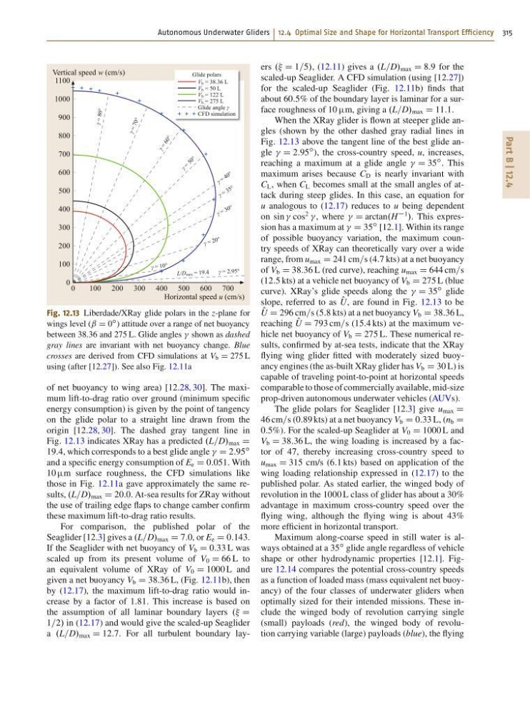
Fig. 12.13 Liberdade/XRay glide polars in the z-plane for
wings level (ˇ D 0
ı ) attitude over a range of net buoyancy
between 38.36 and 275 L. Glide angles shown as dashed
gray lines are invariant with net buoyancy change. Blue
crosses are derived from CFD simulations at V b D 275 L
using (after [12.27]). See also Fig. 12.11a
of net buoyancy to wing area) [12.28, 30]. The maximum lift-to-drag ratio over ground (minimum specific
energy consumption) is given by the point of tangency
on the glide polar to a straight line drawn from the
origin [12.28, 30]. The dashed gray tangent line in
Fig. 12.13 indicates XRay has a predicted .L=D/ max D
19:4, which corresponds to a best glide angle D 2:95
ı
and a specific energy consumption of E e D 0:051. With
10 m surface roughness, the CFD simulations like
those in Fig. 12.11a gave approximately the same results, .L=D/ max D 20:0. At-sea results for ZRay without
the use of trailing edge flaps to change camber confirm
these maximum lift-to-drag ratio results.
For comparison, the published polar of the
Seaglider [12.3] gives a .L=D/ max D 7:0, or E e D 0:143.
If the Seaglider with net buoyancy of V b D 0:33 L was
scaled up from its present volume of V 0 D 66 L to
an equivalent volume of XRay of V 0 D 1000 L and
given a net buoyancy V b D 38:36 L, (Fig. 12.11b), then
by (12.17), the maximum lift-to-drag ratio would increase by a factor of 1:81. This increase is based on
the assumption of all laminar boundary layers .. D
1=2/ in (12.17) and would give the scaled-up Seaglider
a .L=D/ max D 12:7. For all turbulent boundary layers .. D 1=5/, (12.11) gives a .L=D/ max D 8:9 for the
scaled-up Seaglider. A CFD simulation (using [12.27])
for the scaled-up Seaglider (Fig. 12.11b) finds that
about 60:5% of the boundary layer is laminar for a surface roughness of 10 m, giving a .L=D/ max D 11:1.
When the XRay glider is flown at steeper glide angles (shown by the other dashed gray radial lines in
Fig. 12.13 above the tangent line of the best glide angle D 2:95
ı ), the cross-country speed, u, increases,
reaching a maximum at a glide angle D 35
ı . This
maximum arises because C D is nearly invariant with
C L , when C L becomes small at the small angles of attack during steep glides. In this case, an equation for
u analogous to (12.17) reduces to u being dependent
on sin cos
2
, where D arctan.H
1
/. This expression has a maximum at D 35
ı [12.1]. Within its range
of possible buoyancy variation, the maximum country speeds of XRay can theoretically vary over a wide
range, from u max D 241 cm=s (4:7 kts) at a net buoyancy
of V b D 38:36 L (red curve), reaching u max D 644 cm=s
(12:5 kts) at a vehicle net buoyancy of V b D 275 L (blue
curve). XRay’s glide speeds along the D 35
ı glide
slope, referred to as O
U, are found in Fig. 12.13 to be
O
U D 296 cm=s (5:8 kts) at a net buoyancy V b D 38:36 L,
reaching O
U D 793 cm=s (15:4 kts) at the maximum vehicle net buoyancy of V b D 275 L. These numerical results, confirmed by at-sea tests, indicate that the XRay
flying wing glider fitted with moderately sized buoyancy engines (the as-built XRay glider has V b D 30 L) is
capable of traveling point-to-point at horizontal speeds
comparable to those of commercially available, mid-size
prop-driven autonomous underwater vehicles (AUVs).
The glide polars for Seaglider [12.3] give u max D
46 cm=s (0:89 kts) at a net buoyancy V b D 0:33 L, (n b D
0:5%). For the scaled-up Seaglider at V 0 D 1000 L and
V b D 38:36 L, the wing loading is increased by a factor of 47, thereby increasing cross-country speed to
u max D 315 cm/s (6:1 kts) based on application of the
wing loading relationship expressed in (12.17) to the
published polar. As stated earlier, the winged body of
revolution in the 1000 L class of glider has about a 30%
advantage in maximum cross-country speed over the
flying wing, although the flying wing is about 43%
more efficient in horizontal transport.
Maximum along-coarse speed in still water is always obtained at a 35
ı glide angle regardless of vehicle
shape or other hydrodynamic properties [12.1]. Figure 12.14 compares the potential cross-country speeds
as a function of loaded mass (mass equivalent net buoyancy) of the four classes of underwater gliders when
optimally sized for their intended missions. These include the winged body of revolution carrying single
(small) payloads (red), the winged body of revolution carrying variable (large) payloads (blue), the flying
Part B | 12.4
Vb = 38.36 L
Vb = 50 L
Vb = 122 L
Vb = 275 L
Glide angle γ
CFD simulation
Glide polars
0
100 200 300 400 500 600
γ = 2.95°
γ = 10°
γ = 20 °
γ = 3 0 °
γ = 3 5 °
γ = 4 0 °
γ =
5 0 °
γ = 6 0 °
γ = 7 0 °
γ = 80 °
L/Dmax = 19.4
700
Vertical speed w (cm/s)
Horizontal speed u (cm/s)
1100
1000
900
800
700
600
500
400
300
200
100
0
Fig. 12.13 Liberdade/XRay glide polars in the z-plane for
wings level (ˇ D 0
ı ) attitude over a range of net buoyancy
between 38.36 and 275 L. Glide angles shown as dashed
gray lines are invariant with net buoyancy change. Blue
crosses are derived from CFD simulations at V b D 275 L
using (after [12.27]). See also Fig. 12.11a
of net buoyancy to wing area) [12.28, 30]. The maximum lift-to-drag ratio over ground (minimum specific
energy consumption) is given by the point of tangency
on the glide polar to a straight line drawn from the
origin [12.28, 30]. The dashed gray tangent line in
Fig. 12.13 indicates XRay has a predicted .L=D/ max D
19:4, which corresponds to a best glide angle D 2:95
ı
and a specific energy consumption of E e D 0:051. With
10 m surface roughness, the CFD simulations like
those in Fig. 12.11a gave approximately the same results, .L=D/ max D 20:0. At-sea results for ZRay without
the use of trailing edge flaps to change camber confirm
these maximum lift-to-drag ratio results.
For comparison, the published polar of the
Seaglider [12.3] gives a .L=D/ max D 7:0, or E e D 0:143.
If the Seaglider with net buoyancy of V b D 0:33 L was
scaled up from its present volume of V 0 D 66 L to
an equivalent volume of XRay of V 0 D 1000 L and
given a net buoyancy V b D 38:36 L, (Fig. 12.11b), then
by (12.17), the maximum lift-to-drag ratio would increase by a factor of 1:81. This increase is based on
the assumption of all laminar boundary layers .. D
1=2/ in (12.17) and would give the scaled-up Seaglider
a .L=D/ max D 12:7. For all turbulent boundary layers .. D 1=5/, (12.11) gives a .L=D/ max D 8:9 for the
scaled-up Seaglider. A CFD simulation (using [12.27])
for the scaled-up Seaglider (Fig. 12.11b) finds that
about 60:5% of the boundary layer is laminar for a surface roughness of 10 m, giving a .L=D/ max D 11:1.
When the XRay glider is flown at steeper glide angles (shown by the other dashed gray radial lines in
Fig. 12.13 above the tangent line of the best glide angle D 2:95
ı ), the cross-country speed, u, increases,
reaching a maximum at a glide angle D 35
ı . This
maximum arises because C D is nearly invariant with
C L , when C L becomes small at the small angles of attack during steep glides. In this case, an equation for
u analogous to (12.17) reduces to u being dependent
on sin cos
2
, where D arctan.H
1
/. This expression has a maximum at D 35
ı [12.1]. Within its range
of possible buoyancy variation, the maximum country speeds of XRay can theoretically vary over a wide
range, from u max D 241 cm=s (4:7 kts) at a net buoyancy
of V b D 38:36 L (red curve), reaching u max D 644 cm=s
(12:5 kts) at a vehicle net buoyancy of V b D 275 L (blue
curve). XRay’s glide speeds along the D 35
ı glide
slope, referred to as O
U, are found in Fig. 12.13 to be
O
U D 296 cm=s (5:8 kts) at a net buoyancy V b D 38:36 L,
reaching O
U D 793 cm=s (15:4 kts) at the maximum vehicle net buoyancy of V b D 275 L. These numerical results, confirmed by at-sea tests, indicate that the XRay
flying wing glider fitted with moderately sized buoyancy engines (the as-built XRay glider has V b D 30 L) is
capable of traveling point-to-point at horizontal speeds
comparable to those of commercially available, mid-size
prop-driven autonomous underwater vehicles (AUVs).
The glide polars for Seaglider [12.3] give u max D
46 cm=s (0:89 kts) at a net buoyancy V b D 0:33 L, (n b D
0:5%). For the scaled-up Seaglider at V 0 D 1000 L and
V b D 38:36 L, the wing loading is increased by a factor of 47, thereby increasing cross-country speed to
u max D 315 cm/s (6:1 kts) based on application of the
wing loading relationship expressed in (12.17) to the
published polar. As stated earlier, the winged body of
revolution in the 1000 L class of glider has about a 30%
advantage in maximum cross-country speed over the
flying wing, although the flying wing is about 43%
more efficient in horizontal transport.
Maximum along-coarse speed in still water is always obtained at a 35
ı glide angle regardless of vehicle
shape or other hydrodynamic properties [12.1]. Figure 12.14 compares the potential cross-country speeds
as a function of loaded mass (mass equivalent net buoyancy) of the four classes of underwater gliders when
optimally sized for their intended missions. These include the winged body of revolution carrying single
(small) payloads (red), the winged body of revolution carrying variable (large) payloads (blue), the flying