

Part A | 10.5
274 Part A Fundamentals
–10 0
10 20 30 40 50 60 70 80 90
Heading error (rad)
Time (s)
0.02
0.018
0.016
0.014
0.012
0.01
0.008
0.006
0.004
0.002
0
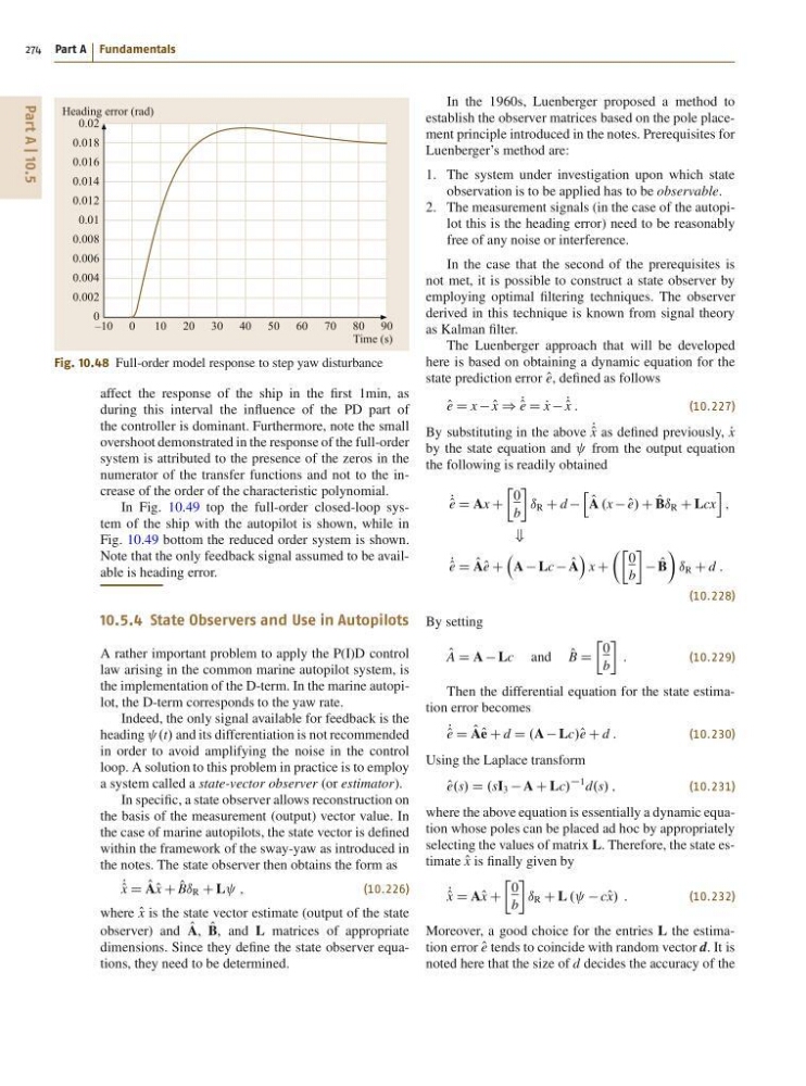
Fig. 10.48 Full-order model response to step yaw disturbance
affect the response of the ship in the first 1min, as
during this interval the influence of the PD part of
the controller is dominant. Furthermore, note the small
overshoot demonstrated in the response of the full-order
system is attributed to the presence of the zeros in the
numerator of the transfer functions and not to the increase of the order of the characteristic polynomial.
In Fig. 10.49 top the full-order closed-loop system of the ship with the autopilot is shown, while in
Fig. 10.49 bottom the reduced order system is shown.
Note that the only feedback signal assumed to be available is heading error.
10.5.4 State Observers and Use in Autopilots
A rather important problem to apply the P(I)D control
law arising in the common marine autopilot system, is
the implementation of the D-term. In the marine autopilot, the D-term corresponds to the yaw rate.
Indeed, the only signal available for feedback is the
heading .t/ and its differentiation is not recommended
in order to avoid amplifying the noise in the control
loop. A solution to this problem in practice is to employ
a system called a state-vector observer (or estimator).
In specific, a state observer allows reconstruction on
the basis of the measurement (output) vector value. In
the case of marine autopilots, the state vector is defined
within the framework of the sway-yaw as introduced in
the notes. The state observer then obtains the form as
P O
x D O
AO x C O
Bı R C L ;
(10.226)
where O
x is the state vector estimate (output of the state
observer) and O
A, O
B, and L matrices of appropriate
dimensions. Since they define the state observer equations, they need to be determined.
In the 1960s, Luenberger proposed a method to
establish the observer matrices based on the pole placement principle introduced in the notes. Prerequisites for
Luenberger’s method are:
1. The system under investigation upon which state
observation is to be applied has to be observable.
2. The measurement signals (in the case of the autopilot this is the heading error) need to be reasonably
free of any noise or interference.
In the case that the second of the prerequisites is
not met, it is possible to construct a state observer by
employing optimal filtering techniques. The observer
derived in this technique is known from signal theory
as Kalman filter.
The Luenberger approach that will be developed
here is based on obtaining a dynamic equation for the
state prediction error O
e, defined as follows
O
e D x O
x ) P O
e D P
x P O
x :
(10.227)
By substituting in the above P O
x as defined previously, P
x
by the state equation and from the output equation
the following is readily obtained
P O
e D Ax C
Ä
0
b
ı R C d
h O
A .x O
e/ C O
Bı R C Lcx
i
;
+
P O
e D O
AO e C
A Lc O
A
Á
x C
ÂÄ
0
b
O
B
Ã
ı R C d :
(10.228)
By setting
O
A D A Lc and O
B D
Ä
0
b
:
(10.229)
Then the differential equation for the state estimation error becomes
P O
e D O
AO e C d D .A Lc/O e C d :
(10.230)
Using the Laplace transform
O
e.s/ D .sI 3 A C Lc/
1 d.s/ ;
(10.231)
where the above equation is essentially a dynamic equation whose poles can be placed ad hoc by appropriately
selecting the values of matrix L. Therefore, the state estimate O
x is finally given by
P O
x D AO x C
Ä
0
b
ı R C L . cO x/ :
(10.232)
Moreover, a good choice for the entries L the estimation error O
e tends to coincide with random vector d. It is
noted here that the size of d decides the accuracy of the
274 Part A Fundamentals
–10 0
10 20 30 40 50 60 70 80 90
Heading error (rad)
Time (s)
0.02
0.018
0.016
0.014
0.012
0.01
0.008
0.006
0.004
0.002
0
Fig. 10.48 Full-order model response to step yaw disturbance
affect the response of the ship in the first 1min, as
during this interval the influence of the PD part of
the controller is dominant. Furthermore, note the small
overshoot demonstrated in the response of the full-order
system is attributed to the presence of the zeros in the
numerator of the transfer functions and not to the increase of the order of the characteristic polynomial.
In Fig. 10.49 top the full-order closed-loop system of the ship with the autopilot is shown, while in
Fig. 10.49 bottom the reduced order system is shown.
Note that the only feedback signal assumed to be available is heading error.
10.5.4 State Observers and Use in Autopilots
A rather important problem to apply the P(I)D control
law arising in the common marine autopilot system, is
the implementation of the D-term. In the marine autopilot, the D-term corresponds to the yaw rate.
Indeed, the only signal available for feedback is the
heading .t/ and its differentiation is not recommended
in order to avoid amplifying the noise in the control
loop. A solution to this problem in practice is to employ
a system called a state-vector observer (or estimator).
In specific, a state observer allows reconstruction on
the basis of the measurement (output) vector value. In
the case of marine autopilots, the state vector is defined
within the framework of the sway-yaw as introduced in
the notes. The state observer then obtains the form as
P O
x D O
AO x C O
Bı R C L ;
(10.226)
where O
x is the state vector estimate (output of the state
observer) and O
A, O
B, and L matrices of appropriate
dimensions. Since they define the state observer equations, they need to be determined.
In the 1960s, Luenberger proposed a method to
establish the observer matrices based on the pole placement principle introduced in the notes. Prerequisites for
Luenberger’s method are:
1. The system under investigation upon which state
observation is to be applied has to be observable.
2. The measurement signals (in the case of the autopilot this is the heading error) need to be reasonably
free of any noise or interference.
In the case that the second of the prerequisites is
not met, it is possible to construct a state observer by
employing optimal filtering techniques. The observer
derived in this technique is known from signal theory
as Kalman filter.
The Luenberger approach that will be developed
here is based on obtaining a dynamic equation for the
state prediction error O
e, defined as follows
O
e D x O
x ) P O
e D P
x P O
x :
(10.227)
By substituting in the above P O
x as defined previously, P
x
by the state equation and from the output equation
the following is readily obtained
P O
e D Ax C
Ä
0
b
ı R C d
h O
A .x O
e/ C O
Bı R C Lcx
i
;
+
P O
e D O
AO e C
A Lc O
A
Á
x C
ÂÄ
0
b
O
B
Ã
ı R C d :
(10.228)
By setting
O
A D A Lc and O
B D
Ä
0
b
:
(10.229)
Then the differential equation for the state estimation error becomes
P O
e D O
AO e C d D .A Lc/O e C d :
(10.230)
Using the Laplace transform
O
e.s/ D .sI 3 A C Lc/
1 d.s/ ;
(10.231)
where the above equation is essentially a dynamic equation whose poles can be placed ad hoc by appropriately
selecting the values of matrix L. Therefore, the state estimate O
x is finally given by
P O
x D AO x C
Ä
0
b
ı R C L . cO x/ :
(10.232)
Moreover, a good choice for the entries L the estimation error O
e tends to coincide with random vector d. It is
noted here that the size of d decides the accuracy of the