

Control Theory and Applications 10.5 Course-Keeping Autopilots 273
Part A | 10.5
Table 10.6 A model for the test case ship maneuvering dynamics
2
4
P
P
v
P
r
3
5 D
2
4
0
0
1
0 0:0279 3:7140
0 0:0005 0:0694
3
5
2
4 v
r
3
5 C
2
4
0
0
0
0:1077 0:5877 10 8 0:0006 10 8
0:0023
0:0002 10 8 C0:0001 10 8
3
5
2
4
ı R
Y 0
N 0
3
5
.s/ D
0:002305s C 0:0001155
s.s 2 C 0:09734s C 0:0001754/
ı R .s/ C
1:518 10 12 s 2:832 10 12
s.s 2 C 0:09734s C 0:0001754/
Y 0 .s/ C
9:43 10 13 s C 2:916 10 14
s.s 2 C 0:09734s C 0:0001754/
N 0 .s/
1 D 555:56s, 2 D 10:47s
0 D 19:96s, Y D 0:54s, N D 32:34s
example, service speed. The above formulas give for
conventional hulls an a priori (before construction of
the full-scale hull) estimation of the ship’s maneuverability.
By using these values the major hydrodynamic
derivatives have been calculated as in Table 10.6.
Finally, the state-space model of the ship for service
speed of 24:4 kn is obtained and thereof the Nomoto
transfer functions are calculated. The results are shown
in Table 10.7. The values for the time constants in
(10.197) and (10.199) are shown in the same table, as
well.
From the values shown in Table 10.7, it is seen that
the value of 1 is one order of magnitude larger than
the values of all other time constants. This is typical
for the hull forms used in the vast majority of merchant
vessels. In specific, the hydrodynamic derivatives obtain such values that instead of the third order Nomoto
transfer functions, the reduced (second) order ones in
(10.202) may be used for control design. Then, as explained for practical automatic pilot applications, a PD
control law can be, under general assumptions, considered, especially for disturbance rejection.
Eventually, a closed-loop transfer function, Q
G
0
N .s/,
connecting yaw disturbance to heading deflection is derived as in (10.204); a similar governs the effect of sway
disturbance on heading.
The objective of disturbance rejection is to make
sure that for the worst case scenario disturbance the induced heading fluctuation lies below specified levels. In
this case, this can be assured, if transfer function Q
G
0
N .s/
is matched to the following form
G.s/ D
k 0 !
2
0
s 2 C 2! 0 s C !
2
0
(10.223)
with
k 0 D 0:0175 10
9 rad=.N m/ ;
! 0 D 0:1308 rad ; s; ; D 1:0 :
(10.224)
Then a sinusoidal turning torque N 0 at any frequency
and with amplitude not exceeding 10
9 N m will result
to a sinusoidal heading error of the same frequency
and with amplitude not exceeding 1
ı
D 0:0175 rad. To
Table 10.7 Estimated values for the ship’s hydrodynamic
derivatives
Y P
v D D8:2534 10 7 kg
Y P r D D1:0752 10
9 kg m
N P
v D D2:7437 10 8 kg m
N P r D D4:2223 10 11 kg m 2
Y v D D5:2709 10 6 kg=s
Y r D 3:9997 10 8 kg m=s
N v D D5:1196 10 8 kg m=s
N r D D7:4747 10 10 kg m 2 =s
Y ı D D1:5878 10 7 N
N ı D 2:4190 10 9 N m
–10 0
10 20 30 40 50 60 70 80 90
Heading error (rad)
Time (s)
0.018
0.016
0.014
0.012
0.01
0.008
0.006
0.004
0.002
0
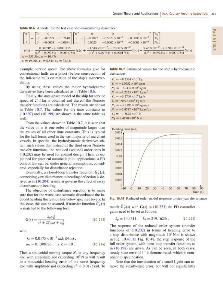
Fig. 10.47 Reduced-order model response to step yaw disturbance
match Q
G
0
N .s/ with G.s/ in (10.223) the PD controller
gains need to be set as follows
k p D 14:4311 ; k d D 219:1623s :
(10.225)
The response of the reduced order system (transfer
functions of (10.202) in terms of heading error to
a step disturbance with magnitude 10
9 N m is shown
in Fig. 10.47. In Fig. 10.48, the step response of the
full order system, with open-loop transfer functions as
in (10.198) are given. As can be seen, in both cases,
steady-state error of 1
ı is demonstrated, which is compliant to specification.
Note that the introduction of a small I-gain can remove the steady-state error, but will not significantly
Part A | 10.5
Table 10.6 A model for the test case ship maneuvering dynamics
2
4
P
P
v
P
r
3
5 D
2
4
0
0
1
0 0:0279 3:7140
0 0:0005 0:0694
3
5
2
4 v
r
3
5 C
2
4
0
0
0
0:1077 0:5877 10 8 0:0006 10 8
0:0023
0:0002 10 8 C0:0001 10 8
3
5
2
4
ı R
Y 0
N 0
3
5
.s/ D
0:002305s C 0:0001155
s.s 2 C 0:09734s C 0:0001754/
ı R .s/ C
1:518 10 12 s 2:832 10 12
s.s 2 C 0:09734s C 0:0001754/
Y 0 .s/ C
9:43 10 13 s C 2:916 10 14
s.s 2 C 0:09734s C 0:0001754/
N 0 .s/
1 D 555:56s, 2 D 10:47s
0 D 19:96s, Y D 0:54s, N D 32:34s
example, service speed. The above formulas give for
conventional hulls an a priori (before construction of
the full-scale hull) estimation of the ship’s maneuverability.
By using these values the major hydrodynamic
derivatives have been calculated as in Table 10.6.
Finally, the state-space model of the ship for service
speed of 24:4 kn is obtained and thereof the Nomoto
transfer functions are calculated. The results are shown
in Table 10.7. The values for the time constants in
(10.197) and (10.199) are shown in the same table, as
well.
From the values shown in Table 10.7, it is seen that
the value of 1 is one order of magnitude larger than
the values of all other time constants. This is typical
for the hull forms used in the vast majority of merchant
vessels. In specific, the hydrodynamic derivatives obtain such values that instead of the third order Nomoto
transfer functions, the reduced (second) order ones in
(10.202) may be used for control design. Then, as explained for practical automatic pilot applications, a PD
control law can be, under general assumptions, considered, especially for disturbance rejection.
Eventually, a closed-loop transfer function, Q
G
0
N .s/,
connecting yaw disturbance to heading deflection is derived as in (10.204); a similar governs the effect of sway
disturbance on heading.
The objective of disturbance rejection is to make
sure that for the worst case scenario disturbance the induced heading fluctuation lies below specified levels. In
this case, this can be assured, if transfer function Q
G
0
N .s/
is matched to the following form
G.s/ D
k 0 !
2
0
s 2 C 2! 0 s C !
2
0
(10.223)
with
k 0 D 0:0175 10
9 rad=.N m/ ;
! 0 D 0:1308 rad ; s; ; D 1:0 :
(10.224)
Then a sinusoidal turning torque N 0 at any frequency
and with amplitude not exceeding 10
9 N m will result
to a sinusoidal heading error of the same frequency
and with amplitude not exceeding 1
ı
D 0:0175 rad. To
Table 10.7 Estimated values for the ship’s hydrodynamic
derivatives
Y P
v D D8:2534 10 7 kg
Y P r D D1:0752 10
9 kg m
N P
v D D2:7437 10 8 kg m
N P r D D4:2223 10 11 kg m 2
Y v D D5:2709 10 6 kg=s
Y r D 3:9997 10 8 kg m=s
N v D D5:1196 10 8 kg m=s
N r D D7:4747 10 10 kg m 2 =s
Y ı D D1:5878 10 7 N
N ı D 2:4190 10 9 N m
–10 0
10 20 30 40 50 60 70 80 90
Heading error (rad)
Time (s)
0.018
0.016
0.014
0.012
0.01
0.008
0.006
0.004
0.002
0
Fig. 10.47 Reduced-order model response to step yaw disturbance
match Q
G
0
N .s/ with G.s/ in (10.223) the PD controller
gains need to be set as follows
k p D 14:4311 ; k d D 219:1623s :
(10.225)
The response of the reduced order system (transfer
functions of (10.202) in terms of heading error to
a step disturbance with magnitude 10
9 N m is shown
in Fig. 10.47. In Fig. 10.48, the step response of the
full order system, with open-loop transfer functions as
in (10.198) are given. As can be seen, in both cases,
steady-state error of 1
ı is demonstrated, which is compliant to specification.
Note that the introduction of a small I-gain can remove the steady-state error, but will not significantly