

Control Theory and Applications 10.5 Course-Keeping Autopilots 267
Part A | 10.5
Then, the determinant jsI n A BFj is calculated. This
determinant is the closed-loop characteristic polynomial p c .s/ of order 3. The coefficients of p c .s/ are
parameterized by the elements of F, F ij . By equating the
coefficients of polynomials p c .s/ and O
p c .s/ and solving
the resulting linear algebraic system of equations, a matrix F is computed as follows
F D
Ä
0:3021 1:4785 0:617
2:4378 0:9649 1:2816
:
(10.175)
The closed-loop transfer function matrix of the
system with feedback matrix F as in (10.175) is as
follows
H.s/ D
2
6
6
6
6
6
6
6
4
s
2
C 1:217s C 0:2183
s 3 C 3s 2 C 2:75s C 0:75
s
2
C 1:595s C 0:4767
s 3 C 3s 2 C 2:75s C 0:75
s
2
1:281s 2:282
s 3 C 3s 2 C 2:75s C 0:75
1:685s 1:549
s 3 C 3s 2 C 2:75s C 0:75
1:403s 1:399
s 3 C 3s 2 C 2:75s C 0:75
s
2
C 1:281s C 0:03623
s 3 C 3s 2 C 2:75s C 0:75
3
7
7
7
7
7
7
7
5
3
:
(10.176)
4
8
1 2
0
4
From: U(1)
From: U(2)
8
1 2
To: Y(1)
Amplitude
Time (s)
0
Time (s)
1
0.5
0
To: Y(2)
2
0
–2
–4
To: Y(3)
1
0
–1
–2
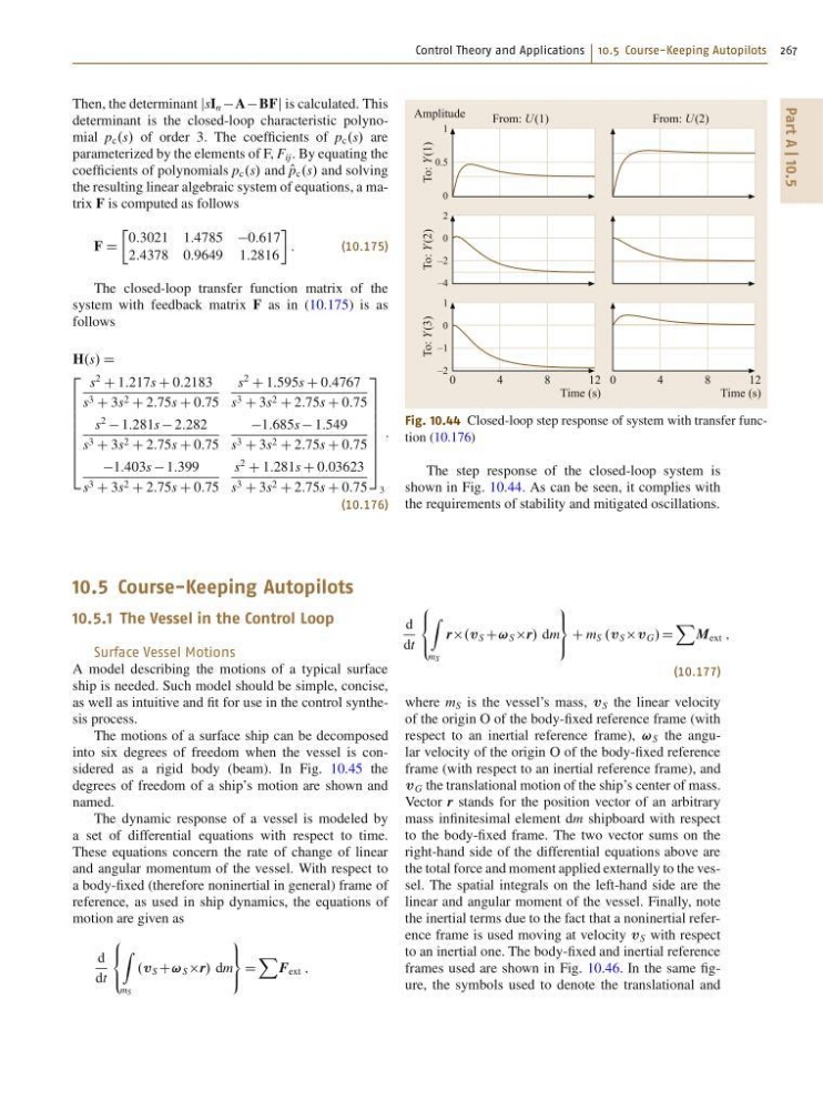
Fig. 10.44 Closed-loop step response of system with transfer function (10.176)
The step response of the closed-loop system is
shown in Fig. 10.44. As can be seen, it complies with
the requirements of stability and mitigated oscillations.
10.5 Course-Keeping Autopilots
10.5.1 The Vessel in the Control Loop
Surface Vessel Motions
A model describing the motions of a typical surface
ship is needed. Such model should be simple, concise,
as well as intuitive and fit for use in the control synthesis process.
The motions of a surface ship can be decomposed
into six degrees of freedom when the vessel is considered as a rigid body (beam). In Fig. 10.45 the
degrees of freedom of a ship’s motion are shown and
named.
The dynamic response of a vessel is modeled by
a set of differential equations with respect to time.
These equations concern the rate of change of linear
and angular momentum of the vessel. With respect to
a body-fixed (therefore noninertial in general) frame of
reference, as used in ship dynamics, the equations of
motion are given as
d
dt
8
<
:
Z
mS
.v S C! S r/ dm
9
=
;
D
X
F ext ;
d
dt
8
<
:
Z
mS
r.v S C! S r/ dm
9
=
;
C m S .v S v G / D
X
M ext ;
(10.177)
where m S is the vessel’s mass, v S the linear velocity
of the origin O of the body-fixed reference frame (with
respect to an inertial reference frame), ! S the angular velocity of the origin O of the body-fixed reference
frame (with respect to an inertial reference frame), and
v G the translational motion of the ship’s center of mass.
Vector r stands for the position vector of an arbitrary
mass infinitesimal element dm shipboard with respect
to the body-fixed frame. The two vector sums on the
right-hand side of the differential equations above are
the total force and moment applied externally to the vessel. The spatial integrals on the left-hand side are the
linear and angular moment of the vessel. Finally, note
the inertial terms due to the fact that a noninertial reference frame is used moving at velocity v S with respect
to an inertial one. The body-fixed and inertial reference
frames used are shown in Fig. 10.46. In the same figure, the symbols used to denote the translational and
Part A | 10.5
Then, the determinant jsI n A BFj is calculated. This
determinant is the closed-loop characteristic polynomial p c .s/ of order 3. The coefficients of p c .s/ are
parameterized by the elements of F, F ij . By equating the
coefficients of polynomials p c .s/ and O
p c .s/ and solving
the resulting linear algebraic system of equations, a matrix F is computed as follows
F D
Ä
0:3021 1:4785 0:617
2:4378 0:9649 1:2816
:
(10.175)
The closed-loop transfer function matrix of the
system with feedback matrix F as in (10.175) is as
follows
H.s/ D
2
6
6
6
6
6
6
6
4
s
2
C 1:217s C 0:2183
s 3 C 3s 2 C 2:75s C 0:75
s
2
C 1:595s C 0:4767
s 3 C 3s 2 C 2:75s C 0:75
s
2
1:281s 2:282
s 3 C 3s 2 C 2:75s C 0:75
1:685s 1:549
s 3 C 3s 2 C 2:75s C 0:75
1:403s 1:399
s 3 C 3s 2 C 2:75s C 0:75
s
2
C 1:281s C 0:03623
s 3 C 3s 2 C 2:75s C 0:75
3
7
7
7
7
7
7
7
5
3
:
(10.176)
4
8
1 2
0
4
From: U(1)
From: U(2)
8
1 2
To: Y(1)
Amplitude
Time (s)
0
Time (s)
1
0.5
0
To: Y(2)
2
0
–2
–4
To: Y(3)
1
0
–1
–2
Fig. 10.44 Closed-loop step response of system with transfer function (10.176)
The step response of the closed-loop system is
shown in Fig. 10.44. As can be seen, it complies with
the requirements of stability and mitigated oscillations.
10.5 Course-Keeping Autopilots
10.5.1 The Vessel in the Control Loop
Surface Vessel Motions
A model describing the motions of a typical surface
ship is needed. Such model should be simple, concise,
as well as intuitive and fit for use in the control synthesis process.
The motions of a surface ship can be decomposed
into six degrees of freedom when the vessel is considered as a rigid body (beam). In Fig. 10.45 the
degrees of freedom of a ship’s motion are shown and
named.
The dynamic response of a vessel is modeled by
a set of differential equations with respect to time.
These equations concern the rate of change of linear
and angular momentum of the vessel. With respect to
a body-fixed (therefore noninertial in general) frame of
reference, as used in ship dynamics, the equations of
motion are given as
d
dt
8
<
:
Z
mS
.v S C! S r/ dm
9
=
;
D
X
F ext ;
d
dt
8
<
:
Z
mS
r.v S C! S r/ dm
9
=
;
C m S .v S v G / D
X
M ext ;
(10.177)
where m S is the vessel’s mass, v S the linear velocity
of the origin O of the body-fixed reference frame (with
respect to an inertial reference frame), ! S the angular velocity of the origin O of the body-fixed reference
frame (with respect to an inertial reference frame), and
v G the translational motion of the ship’s center of mass.
Vector r stands for the position vector of an arbitrary
mass infinitesimal element dm shipboard with respect
to the body-fixed frame. The two vector sums on the
right-hand side of the differential equations above are
the total force and moment applied externally to the vessel. The spatial integrals on the left-hand side are the
linear and angular moment of the vessel. Finally, note
the inertial terms due to the fact that a noninertial reference frame is used moving at velocity v S with respect
to an inertial one. The body-fixed and inertial reference
frames used are shown in Fig. 10.46. In the same figure, the symbols used to denote the translational and