

Part A | 10.4
266 Part A Fundamentals
–1 –0.8 –0.6 –0.4 –0.2 0 0.2 0.4 0.6 0.8 1
Imag axis
Real axis
2.5
2
1.5
1
0.5
0
–0.5
–1
–1.5
–2
–2.5
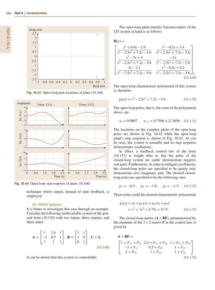
Fig. 10.42 Open-loop pole locations of plant (10.168)
0
0.6
1.2
From: U(1)
From: U (2)
1.8
2.4
To: Y(1)
Amplitude
Time (s)
0
0.6
1.2
1.8
2.4
Time (s)
4
2
0
–2
–4
To: Y(2)
5
0
–5
To: Y(3)
10
5
0
–5
Fig. 10.43 Open-loop step response of plant (10.168)
technique where output, instead of state feedback, is
employed.
LTI–MIMO Systems
It is better to investigate this case through an example.
Consider the following multivariable system of the general form (10.154) with two inputs, three outputs, and
three states
A D
2
4
1 2:4 1
3 0:5 1
1
1 1
3
5 ; B D
2
4
1 1
1 0
0 1
3
5 ; C D I 3 :
(10.168)
It can be shown that this system is controllable.
The open-loop plant transfer function matrix of the
LTI system at hand is as follows
H.s/ D
2
6
6
6
6
6
6
6
4
s
2
C 0:9s 1:9
s 3 2:5s 2 C 7:2s 5:6
s
2
0:5s C 1:4
s 3 2:5s 2 C 7:2s 5:6
s
2
5s C 4
s 3 2:5s 2 C 7:2s 5:6
2s
s 3 2:5s 2 C 7:2s 5:6
2s 2:1
s 3 2:5s 2 C 7:2s 5:6
s
2
0:5s C 4:2
s 3 2:5s 2 C 7:2s 5:6
3
7
7
7
7
7
7
7
5
3
:
(10.169)
The open-loop characteristic polynomial of this system
is, therefore
p 0 .s/ D s
3
2:5s
2
C 7:2s 5:6 :
(10.170)
The open-loop poles, that is, the roots of the polynomial
above, are
s 0 D 0:9807 ; s 1;2 D 0:7596 ˙ i2:2656 : (10.171)
The locations on the complex plane of the open-loop
poles are shown in Fig. 10.42 while the open-loop
plant’s step response is shown in Fig. 10.43. As can
be seen, the system is unstable and its step response
demonstrates oscillations.
In effect, a feedback control law of the form
(10.157) is sought after so that the poles of the
closed-loop system are stable (demonstrate negative
real part). Furthermore, in order to mitigate oscillations,
the closed-loop poles are specified to be purely real,
demonstrate zero imaginary part. The desired closedloop poles are specified to be the following ones
p 1 D D0:5 ; p 2 D D1:0 ; p 3 D D1:5 : (10.172)
These poles yield the desired characteristic polynomial
O
p c .s/ D .s C p 1 / .s C p 2 / .s C p 3 /
D s
3
C 3s
2
C 2:75s C 0:75 :
(10.173)
The closed-loop matrix (A C BF), parameterized by
the elements of the 3 2 matrix F in the control law, is
given by
A C BF D
2
4
1 C F 11 C F 21 2:4 C F 12 C F 22 1 C F 13 C F 23
3 C F 11
0:5 C F 12
1 C F 13
1 C F 21
1 C F 22
1 C F 23
3
5 :
(10.174)
266 Part A Fundamentals
–1 –0.8 –0.6 –0.4 –0.2 0 0.2 0.4 0.6 0.8 1
Imag axis
Real axis
2.5
2
1.5
1
0.5
0
–0.5
–1
–1.5
–2
–2.5
Fig. 10.42 Open-loop pole locations of plant (10.168)
0
0.6
1.2
From: U(1)
From: U (2)
1.8
2.4
To: Y(1)
Amplitude
Time (s)
0
0.6
1.2
1.8
2.4
Time (s)
4
2
0
–2
–4
To: Y(2)
5
0
–5
To: Y(3)
10
5
0
–5
Fig. 10.43 Open-loop step response of plant (10.168)
technique where output, instead of state feedback, is
employed.
LTI–MIMO Systems
It is better to investigate this case through an example.
Consider the following multivariable system of the general form (10.154) with two inputs, three outputs, and
three states
A D
2
4
1 2:4 1
3 0:5 1
1
1 1
3
5 ; B D
2
4
1 1
1 0
0 1
3
5 ; C D I 3 :
(10.168)
It can be shown that this system is controllable.
The open-loop plant transfer function matrix of the
LTI system at hand is as follows
H.s/ D
2
6
6
6
6
6
6
6
4
s
2
C 0:9s 1:9
s 3 2:5s 2 C 7:2s 5:6
s
2
0:5s C 1:4
s 3 2:5s 2 C 7:2s 5:6
s
2
5s C 4
s 3 2:5s 2 C 7:2s 5:6
2s
s 3 2:5s 2 C 7:2s 5:6
2s 2:1
s 3 2:5s 2 C 7:2s 5:6
s
2
0:5s C 4:2
s 3 2:5s 2 C 7:2s 5:6
3
7
7
7
7
7
7
7
5
3
:
(10.169)
The open-loop characteristic polynomial of this system
is, therefore
p 0 .s/ D s
3
2:5s
2
C 7:2s 5:6 :
(10.170)
The open-loop poles, that is, the roots of the polynomial
above, are
s 0 D 0:9807 ; s 1;2 D 0:7596 ˙ i2:2656 : (10.171)
The locations on the complex plane of the open-loop
poles are shown in Fig. 10.42 while the open-loop
plant’s step response is shown in Fig. 10.43. As can
be seen, the system is unstable and its step response
demonstrates oscillations.
In effect, a feedback control law of the form
(10.157) is sought after so that the poles of the
closed-loop system are stable (demonstrate negative
real part). Furthermore, in order to mitigate oscillations,
the closed-loop poles are specified to be purely real,
demonstrate zero imaginary part. The desired closedloop poles are specified to be the following ones
p 1 D D0:5 ; p 2 D D1:0 ; p 3 D D1:5 : (10.172)
These poles yield the desired characteristic polynomial
O
p c .s/ D .s C p 1 / .s C p 2 / .s C p 3 /
D s
3
C 3s
2
C 2:75s C 0:75 :
(10.173)
The closed-loop matrix (A C BF), parameterized by
the elements of the 3 2 matrix F in the control law, is
given by
A C BF D
2
4
1 C F 11 C F 21 2:4 C F 12 C F 22 1 C F 13 C F 23
3 C F 11
0:5 C F 12
1 C F 13
1 C F 21
1 C F 22
1 C F 23
3
5 :
(10.174)