

Control Theory and Applications 10.4 Pole Placement of LTI Systems 265
Part A | 10.4
be directly obtained as follows
p c .s/ D jsI n A BFj
D s
n
C a n1 s
n1
C C C C C a 1 s C a 0
(10.161)
In (10.161), the coefficients of polynomial p c .s/ are
functions of the elements in the m n feedback matrix
F. Furthermore, for the pole placement problem it can
be assumed that m D m r and L D I m .
The specifications in a pole placement problem consist of the desired locations of the closed-loop poles
on the complex plane. As mentioned before, physically realizable systems, that is, with real parameters,
have either purely real poles or pairs of complex conjugate poles. Therefore, in the factorized form of the
characteristic polynomial of any physically realizable
system, a purely real pole p corresponds to a factor
of the form .s p/ while a pair of complex conjugate poles p and p
corresponds to the second-order
factor .s p/.s p
/ D s
2
2Re.p/s C jpj
2 . By multiplicatively combining all such factors corresponding to
the desired closed-loop poles and algebraically manipulating their product, a polynomial in reduced form like
O
p c .s/ D s
n
C O
a n1 s
n1
C C C C C O
a 1 s C O
a 0 is obtained.
Then, one has to equate the coefficients of the same
powers of s of polynomials p c .s/ and O
p c .s/. By doing
that, a linear algebraic system of n equations is obtained, which if solved provides for the constants in the
feedback matrix F of the controller
a v .F ij I i D 1; : : : ; m; j D 1; : : : ; n/ D O
a v ;
v D 1; : : : ; n :
(10.162)
In general, the number of equations of the algebraic
system above is smaller than the number of unknowns.
This means that after successfully solving the algebraic
system (10.162), there remain .m 1/n (if m > 1) free
design parameters in the controller, to be used in order
to meet objectives other than pole placement.
LTI–SISO Systems in Companion Canonical Form
Pole placement design is now investigated in the case
of an LTI–SISO system with scalar transfer function of
the form shown below.
H.s/ D
Y.s/
U.s/
D
b 0
s n C a n1 s n1 C C C C C a 1 s C a 0
(10.163)
Further, the state-space realization in companion canonical form as in (10.47) is considered. The full-state
feedback matrix F for this realization is, therefore, of
dimensions 1 n and with the general form
F D
f 0 f 1 : : : f n1
:
(10.164)
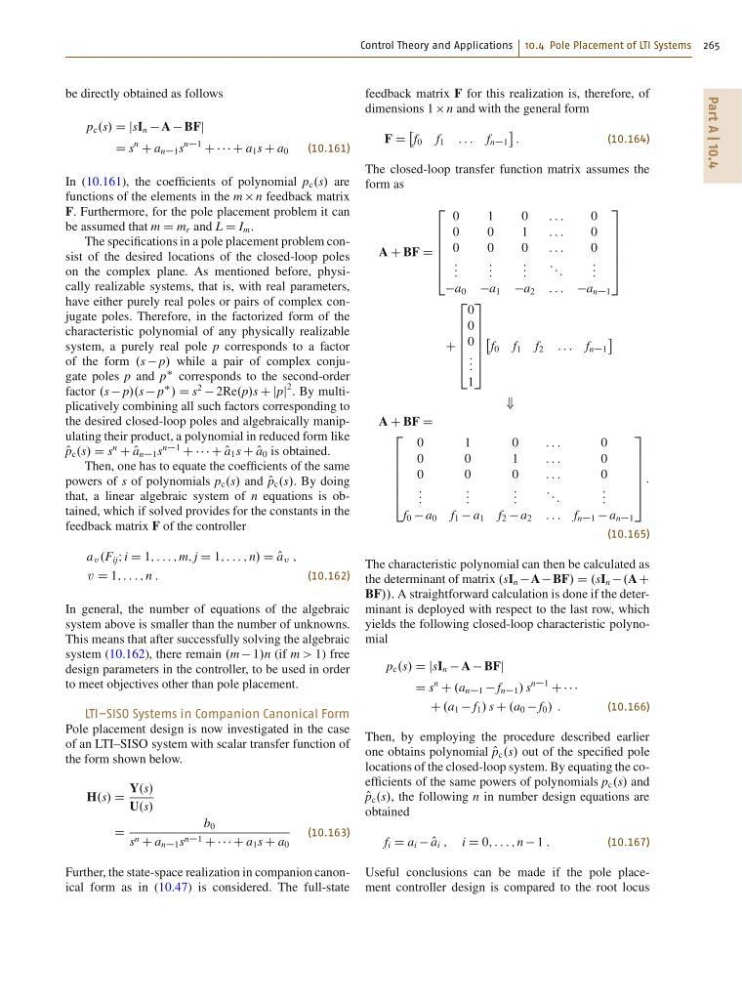
The closed-loop transfer function matrix assumes the
form as
A C BF D
2
6
6
6
6
6
4
0
1
0
: : :
0
0
0
1
: : :
0
0
0
0
: : :
0
: : :
: : :
: : :
: : :
: : :
a 0 a 1 a 2 : : : a n1
3
7
7
7
7
7
5
C
2
6
6
6
6
6
4
0
0
0
: : :
1
3
7
7
7
7
7
5
f 0 f 1 f 2 : : : f n1
+
A C BF D
2
6
6
6
6
6
4
0
1
0
: : :
0
0
0
1
: : :
0
0
0
0
: : :
0
: : :
: : :
: : :
: : :
: : :
f 0 a 0 f 1 a 1 f 2 a 2 : : : f n1 a n1
3
7
7
7
7
7
5
:
(10.165)
The characteristic polynomial can then be calculated as
the determinant of matrix .sI n A BF/ D .sI n .A C
BF//. A straightforward calculation is done if the determinant is deployed with respect to the last row, which
yields the following closed-loop characteristic polynomial
p c .s/ D jsI n A BFj
D s
n
C .a n1 f n1 / s
n1
C C C C
C .a 1 f 1 / s C .a 0 f 0 / :
(10.166)
Then, by employing the procedure described earlier
one obtains polynomial O
p c .s/ out of the specified pole
locations of the closed-loop system. By equating the coefficients of the same powers of polynomials p c .s/ and
O
p c .s/, the following n in number design equations are
obtained
f i D a i O
a i ; i D 0; : : : ; n 1 :
(10.167)
Useful conclusions can be made if the pole placement controller design is compared to the root locus
Part A | 10.4
be directly obtained as follows
p c .s/ D jsI n A BFj
D s
n
C a n1 s
n1
C C C C C a 1 s C a 0
(10.161)
In (10.161), the coefficients of polynomial p c .s/ are
functions of the elements in the m n feedback matrix
F. Furthermore, for the pole placement problem it can
be assumed that m D m r and L D I m .
The specifications in a pole placement problem consist of the desired locations of the closed-loop poles
on the complex plane. As mentioned before, physically realizable systems, that is, with real parameters,
have either purely real poles or pairs of complex conjugate poles. Therefore, in the factorized form of the
characteristic polynomial of any physically realizable
system, a purely real pole p corresponds to a factor
of the form .s p/ while a pair of complex conjugate poles p and p
corresponds to the second-order
factor .s p/.s p
/ D s
2
2Re.p/s C jpj
2 . By multiplicatively combining all such factors corresponding to
the desired closed-loop poles and algebraically manipulating their product, a polynomial in reduced form like
O
p c .s/ D s
n
C O
a n1 s
n1
C C C C C O
a 1 s C O
a 0 is obtained.
Then, one has to equate the coefficients of the same
powers of s of polynomials p c .s/ and O
p c .s/. By doing
that, a linear algebraic system of n equations is obtained, which if solved provides for the constants in the
feedback matrix F of the controller
a v .F ij I i D 1; : : : ; m; j D 1; : : : ; n/ D O
a v ;
v D 1; : : : ; n :
(10.162)
In general, the number of equations of the algebraic
system above is smaller than the number of unknowns.
This means that after successfully solving the algebraic
system (10.162), there remain .m 1/n (if m > 1) free
design parameters in the controller, to be used in order
to meet objectives other than pole placement.
LTI–SISO Systems in Companion Canonical Form
Pole placement design is now investigated in the case
of an LTI–SISO system with scalar transfer function of
the form shown below.
H.s/ D
Y.s/
U.s/
D
b 0
s n C a n1 s n1 C C C C C a 1 s C a 0
(10.163)
Further, the state-space realization in companion canonical form as in (10.47) is considered. The full-state
feedback matrix F for this realization is, therefore, of
dimensions 1 n and with the general form
F D
f 0 f 1 : : : f n1
:
(10.164)
The closed-loop transfer function matrix assumes the
form as
A C BF D
2
6
6
6
6
6
4
0
1
0
: : :
0
0
0
1
: : :
0
0
0
0
: : :
0
: : :
: : :
: : :
: : :
: : :
a 0 a 1 a 2 : : : a n1
3
7
7
7
7
7
5
C
2
6
6
6
6
6
4
0
0
0
: : :
1
3
7
7
7
7
7
5
f 0 f 1 f 2 : : : f n1
+
A C BF D
2
6
6
6
6
6
4
0
1
0
: : :
0
0
0
1
: : :
0
0
0
0
: : :
0
: : :
: : :
: : :
: : :
: : :
f 0 a 0 f 1 a 1 f 2 a 2 : : : f n1 a n1
3
7
7
7
7
7
5
:
(10.165)
The characteristic polynomial can then be calculated as
the determinant of matrix .sI n A BF/ D .sI n .A C
BF//. A straightforward calculation is done if the determinant is deployed with respect to the last row, which
yields the following closed-loop characteristic polynomial
p c .s/ D jsI n A BFj
D s
n
C .a n1 f n1 / s
n1
C C C C
C .a 1 f 1 / s C .a 0 f 0 / :
(10.166)
Then, by employing the procedure described earlier
one obtains polynomial O
p c .s/ out of the specified pole
locations of the closed-loop system. By equating the coefficients of the same powers of polynomials p c .s/ and
O
p c .s/, the following n in number design equations are
obtained
f i D a i O
a i ; i D 0; : : : ; n 1 :
(10.167)
Useful conclusions can be made if the pole placement controller design is compared to the root locus