

Part A | 10.4
264 Part A Fundamentals
1
s
r
y
x
u
+
+
+
+
L
B
I n
C
F
A
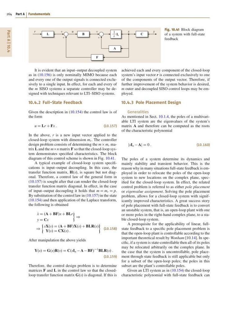
Fig. 10.41 Block diagram
of a system with full-state
feedback
It is evident that an input–output decoupled system
as in (10.156) is only nominally MIMO because each
and every one of the output signals is connected exclusively to a single input. In effect, for each and every of
the m SISO systems a separate controller may be designed with techniques relevant to LTI–SISO systems.
10.4.2 Full-State Feedback
Given the description in (10.154) the control law is of
the form
u D Lr C Fx :
(10.157)
In the above, r is a new input vector applied to the
closed-loop system with dimension m r . The controller
design problem consists of determining the m m r matrix L and the mn matrix F so that the closed-loop system demonstrates specified characteristics. The block
diagram of this control scheme is shown in Fig. 10.41.
A typical example of closed-loop system specifications is input–output decoupling. In this case, the
transfer function matrix, H.s/, is square but not diagonal. Therefore, a control law of the general form in
(10.157) is sought after that can render the closed-loop
transfer function matrix diagonal. In effect, in the case
of input–output decoupling it holds that m D m r D p.
By substitution of the control law in (10.157) in the state
(10.154) and then application of the Laplace transform,
the following is obtained
P
x D .A C BF/x C BLr
y D Cx
)
)
sX.s/ D .A C BF/X.s/ C BLR.s/
Y.s/ D CX.s/ :
(10.158)
After manipulation the above yields
Y.s/ D G.s/R.s/ D C.sI n A BF/
1 BLR.s/ :
(10.159)
Therefore, the control design problem is to determine
matrices F and L in the control law so that the closedloop transfer function matrix G.s/ is diagonal. If this is
achieved each and every component of the closed-loop
system’s input vector r is connected exclusively to one
of the components of the output vector. Therefore, if
further improvement of the system behavior is desired,
m outer and decoupled SISO control loops may be employed.
10.4.3 Pole Placement Design
Generalities
As mentioned in Sect. 10.1.4, the poles of a multivariable LTI system are the eigenvalues of the system’s
matrix A and therefore can be computed as the roots
of the characteristic polynomial
jsI n Aj D 0 :
(10.160)
The poles of a system determine its dynamics and
mainly stability and transient behavior. This is the
reason why in many situations full-state feedback is employed in order to relocate the poles of the open-loop
system to new locations on the complex plane, specified for the closed-loop system. In effect, the related
control problem is referred to as either pole placement
or eigenvalue assignment. Solving the pole placement
problem, allows for a closed-loop system with significantly improved characteristics. A great success story
of pole placement with full-state feedback is to convert
an unstable system, that is, an open-loop plant with one
or more poles in the right-hand complex plane, to a stable closed-loop system.
A prerequisite for the applicability of linear, fullstate feedback to a specific pole placement problem is
that the open-loop plant is controllable according to the
important theoretical result by Wonham [10.14]. In specific, if a system is state-controllable then all of its poles
may be relocated arbitrarily on the complex plane. In
the case that the system is uncontrollable, pole placement through state feedback is still applicable but only
for a subset of the open-loop poles; the poles in this
subset are the plant’s controllable poles.
Given an LTI system as in (10.154) the closed-loop
characteristic polynomial with full-state feedback can
264 Part A Fundamentals
1
s
r
y
x
u
+
+
+
+
L
B
I n
C
F
A
Fig. 10.41 Block diagram
of a system with full-state
feedback
It is evident that an input–output decoupled system
as in (10.156) is only nominally MIMO because each
and every one of the output signals is connected exclusively to a single input. In effect, for each and every of
the m SISO systems a separate controller may be designed with techniques relevant to LTI–SISO systems.
10.4.2 Full-State Feedback
Given the description in (10.154) the control law is of
the form
u D Lr C Fx :
(10.157)
In the above, r is a new input vector applied to the
closed-loop system with dimension m r . The controller
design problem consists of determining the m m r matrix L and the mn matrix F so that the closed-loop system demonstrates specified characteristics. The block
diagram of this control scheme is shown in Fig. 10.41.
A typical example of closed-loop system specifications is input–output decoupling. In this case, the
transfer function matrix, H.s/, is square but not diagonal. Therefore, a control law of the general form in
(10.157) is sought after that can render the closed-loop
transfer function matrix diagonal. In effect, in the case
of input–output decoupling it holds that m D m r D p.
By substitution of the control law in (10.157) in the state
(10.154) and then application of the Laplace transform,
the following is obtained
P
x D .A C BF/x C BLr
y D Cx
)
)
sX.s/ D .A C BF/X.s/ C BLR.s/
Y.s/ D CX.s/ :
(10.158)
After manipulation the above yields
Y.s/ D G.s/R.s/ D C.sI n A BF/
1 BLR.s/ :
(10.159)
Therefore, the control design problem is to determine
matrices F and L in the control law so that the closedloop transfer function matrix G.s/ is diagonal. If this is
achieved each and every component of the closed-loop
system’s input vector r is connected exclusively to one
of the components of the output vector. Therefore, if
further improvement of the system behavior is desired,
m outer and decoupled SISO control loops may be employed.
10.4.3 Pole Placement Design
Generalities
As mentioned in Sect. 10.1.4, the poles of a multivariable LTI system are the eigenvalues of the system’s
matrix A and therefore can be computed as the roots
of the characteristic polynomial
jsI n Aj D 0 :
(10.160)
The poles of a system determine its dynamics and
mainly stability and transient behavior. This is the
reason why in many situations full-state feedback is employed in order to relocate the poles of the open-loop
system to new locations on the complex plane, specified for the closed-loop system. In effect, the related
control problem is referred to as either pole placement
or eigenvalue assignment. Solving the pole placement
problem, allows for a closed-loop system with significantly improved characteristics. A great success story
of pole placement with full-state feedback is to convert
an unstable system, that is, an open-loop plant with one
or more poles in the right-hand complex plane, to a stable closed-loop system.
A prerequisite for the applicability of linear, fullstate feedback to a specific pole placement problem is
that the open-loop plant is controllable according to the
important theoretical result by Wonham [10.14]. In specific, if a system is state-controllable then all of its poles
may be relocated arbitrarily on the complex plane. In
the case that the system is uncontrollable, pole placement through state feedback is still applicable but only
for a subset of the open-loop poles; the poles in this
subset are the plant’s controllable poles.
Given an LTI system as in (10.154) the closed-loop
characteristic polynomial with full-state feedback can