

Control Theory and Applications 10.2 Analysis of LTI Systems 245
Part A | 10.2
Step response (Fig. 10.15)
y step .t/ D 1 e
t cos .! n t/
! n
e
t sin .! n t/
D 1
e
t
p
1 2
sin .! n t C Â/ ;
(10.96)
where
D Re fp 1;2 g D D! 0 and
 D arctan
p
1 2
!
:
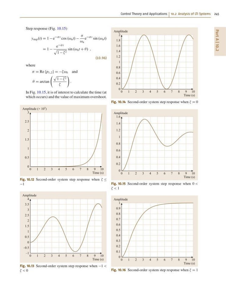
In Fig. 10.15, it is of interest to calculate the time (at
which occurs) and the value of maximum overshoot.
0
1
2
3
4
5
6
7
8
9 10
Amplitude (× 10
5 )
Time (s)
3
2.5
2
1.5
1
0.5
0
Fig. 10.12 Second-order system step response when Ä
1
0
1
2
3
4
5
6
7
8
9 10
Amplitude
Time (s)
4
3.5
3
2.5
2
1.5
1
0.5
0
–0.5
–1
Fig. 10.13 Second-order system step response when 1 <
< 0
0
1
2
3
4
5
6
7
8
9 10
Amplitude
Time (s)
2
1.8
1.6
1.4
1.2
1
0.8
0.6
0.4
0.2
0
Fig. 10.14 Second-order system step response when D 0
0
1
2
3
4
5
6
7
8
9 10
Amplitude
Time (s)
1.6
1.4
1.2
1
0.8
0.6
0.4
0.2
0
Fig. 10.15 Second-order system step response when 0 <
< 1
0
1
2
3
4
5
6
7
8
9 10
Amplitude
Time (s)
1
0.9
0.8
0.7
0.6
0.5
0.4
0.3
0.2
0.1
0
Fig. 10.16 Second-order system step response when D 1
Part A | 10.2
Step response (Fig. 10.15)
y step .t/ D 1 e
t cos .! n t/
! n
e
t sin .! n t/
D 1
e
t
p
1 2
sin .! n t C Â/ ;
(10.96)
where
D Re fp 1;2 g D D! 0 and
 D arctan
p
1 2
!
:
In Fig. 10.15, it is of interest to calculate the time (at
which occurs) and the value of maximum overshoot.
0
1
2
3
4
5
6
7
8
9 10
Amplitude (× 10
5 )
Time (s)
3
2.5
2
1.5
1
0.5
0
Fig. 10.12 Second-order system step response when Ä
1
0
1
2
3
4
5
6
7
8
9 10
Amplitude
Time (s)
4
3.5
3
2.5
2
1.5
1
0.5
0
–0.5
–1
Fig. 10.13 Second-order system step response when 1 <
< 0
0
1
2
3
4
5
6
7
8
9 10
Amplitude
Time (s)
2
1.8
1.6
1.4
1.2
1
0.8
0.6
0.4
0.2
0
Fig. 10.14 Second-order system step response when D 0
0
1
2
3
4
5
6
7
8
9 10
Amplitude
Time (s)
1.6
1.4
1.2
1
0.8
0.6
0.4
0.2
0
Fig. 10.15 Second-order system step response when 0 <
< 1
0
1
2
3
4
5
6
7
8
9 10
Amplitude
Time (s)
1
0.9
0.8
0.7
0.6
0.5
0.4
0.3
0.2
0.1
0
Fig. 10.16 Second-order system step response when D 1