

Part A | 10.2
246 Part A Fundamentals
0
1
2
3
4
5
6
7
8
9 10
Amplitude
Time (s)
1
0.9
0.8
0.7
0.6
0.5
0.4
0.3
0.2
0.1
0
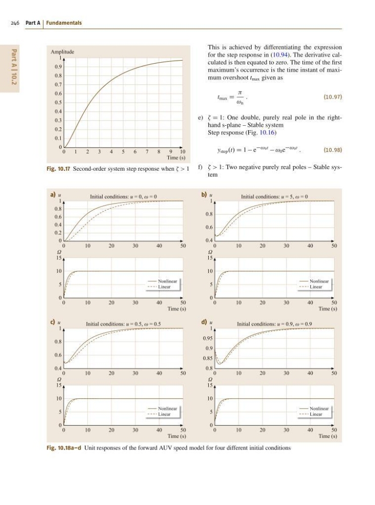
Fig. 10.17 Second-order system step response when > 1
Nonlinear
Linear
Nonlinear
Linear
Nonlinear
Linear
Nonlinear
Linear
a) u
1
0.8
0.6
0.4
0.2
0
0
1 0
2 0
Initial conditions: u = 0, ω = 0
Initial conditions: u = 5, ω = 0
30
40
50
Ω
15
10
5
0
15
10
5
0
0
1 0
2 0
3 0
4 0
5 0
Time (s)
b) u
1
0.8
0.6
0.4
0
1 0
2 0
3 0
4 0
5 0
Ω
0
1 0
2 0
3 0
4 0
5 0
Time (s)
c) u
1
0.8
0.6
0.4 0
1 0
2 0
Initial conditions: u = 0.5, ω = 0.5
Initial conditions: u = 0.9, ω = 0.9
30
40
50
Ω
15
10
5
0
15
10
5
0
0
1 0
2 0
3 0
4 0
5 0
Time (s)
d) u
1
0.95
0.9
0.85
0.8 0
1 0
2 0
3 0
4 0
5 0
Ω
0
1 0
2 0
3 0
4 0
5 0
Time (s)
Fig. 10.18a–d Unit responses of the forward AUV speed model for four different initial conditions
This is achieved by differentiating the expression
for the step response in (10.94). The derivative calculated is then equated to zero. The time of the first
maximum’s occurrence is the time instant of maximum overshoot t max given as
t max D
! n
:
(10.97)
e) D 1: One double, purely real pole in the righthand s-plane – Stable system
Step response (Fig. 10.16)
y step .t/ D 1 e
!0t
! 0 e
!0t
:
(10.98)
f) > 1: Two negative purely real poles – Stable system
246 Part A Fundamentals
0
1
2
3
4
5
6
7
8
9 10
Amplitude
Time (s)
1
0.9
0.8
0.7
0.6
0.5
0.4
0.3
0.2
0.1
0
Fig. 10.17 Second-order system step response when > 1
Nonlinear
Linear
Nonlinear
Linear
Nonlinear
Linear
Nonlinear
Linear
a) u
1
0.8
0.6
0.4
0.2
0
0
1 0
2 0
Initial conditions: u = 0, ω = 0
Initial conditions: u = 5, ω = 0
30
40
50
Ω
15
10
5
0
15
10
5
0
0
1 0
2 0
3 0
4 0
5 0
Time (s)
b) u
1
0.8
0.6
0.4
0
1 0
2 0
3 0
4 0
5 0
Ω
0
1 0
2 0
3 0
4 0
5 0
Time (s)
c) u
1
0.8
0.6
0.4 0
1 0
2 0
Initial conditions: u = 0.5, ω = 0.5
Initial conditions: u = 0.9, ω = 0.9
30
40
50
Ω
15
10
5
0
15
10
5
0
0
1 0
2 0
3 0
4 0
5 0
Time (s)
d) u
1
0.95
0.9
0.85
0.8 0
1 0
2 0
3 0
4 0
5 0
Ω
0
1 0
2 0
3 0
4 0
5 0
Time (s)
Fig. 10.18a–d Unit responses of the forward AUV speed model for four different initial conditions
This is achieved by differentiating the expression
for the step response in (10.94). The derivative calculated is then equated to zero. The time of the first
maximum’s occurrence is the time instant of maximum overshoot t max given as
t max D
! n
:
(10.97)
e) D 1: One double, purely real pole in the righthand s-plane – Stable system
Step response (Fig. 10.16)
y step .t/ D 1 e
!0t
! 0 e
!0t
:
(10.98)
f) > 1: Two negative purely real poles – Stable system