

Part A | 10.2
244 Part A Fundamentals
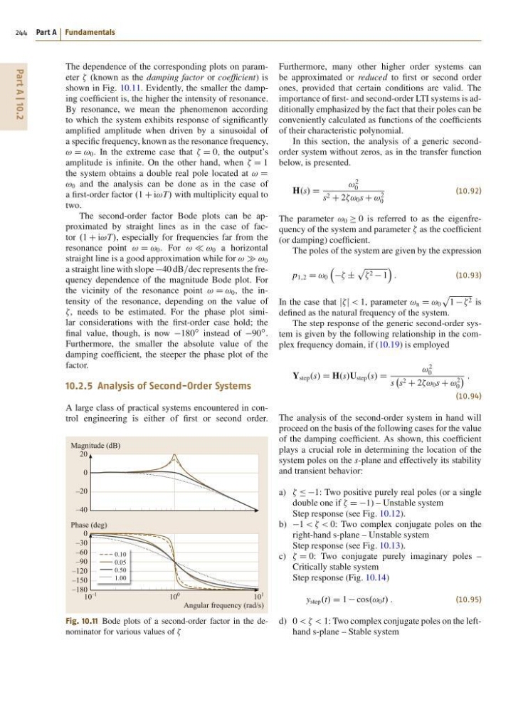
The dependence of the corresponding plots on parameter (known as the damping factor or coefficient) is
shown in Fig. 10.11. Evidently, the smaller the damping coefficient is, the higher the intensity of resonance.
By resonance, we mean the phenomenon according
to which the system exhibits response of significantly
amplified amplitude when driven by a sinusoidal of
a specific frequency, known as the resonance frequency,
! D ! 0 . In the extreme case that D 0, the output’s
amplitude is infinite. On the other hand, when D 1
the system obtains a double real pole located at ! D
! 0 and the analysis can be done as in the case of
a first-order factor .1 C i!T/ with multiplicity equal to
two.
The second-order factor Bode plots can be approximated by straight lines as in the case of factor .1 C i!T/, especially for frequencies far from the
resonance point ! D ! 0 . For ! ! 0 a horizontal
straight line is a good approximation while for ! ! 0
a straight line with slope 40 dB=dec represents the frequency dependence of the magnitude Bode plot. For
the vicinity of the resonance point ! D ! 0 , the intensity of the resonance, depending on the value of
, needs to be estimated. For the phase plot similar considerations with the first-order case hold; the
final value, though, is now 180
ı instead of 90
ı .
Furthermore, the smaller the absolute value of the
damping coefficient, the steeper the phase plot of the
factor.
10.2.5 Analysis of Second-Order Systems
A large class of practical systems encountered in control engineering is either of first or second order.
0.10
0.05
0.50
1.00
Magnitude (dB)
20
0
–20
–40
10
–1
10
0
10
1
Phase (deg)
Angular frequency (rad/s)
0
–30
–60
–90
–120
–150
–180
Fig. 10.11 Bode plots of a second-order factor in the denominator for various values of
Furthermore, many other higher order systems can
be approximated or reduced to first or second order
ones, provided that certain conditions are valid. The
importance of first- and second-order LTI systems is additionally emphasized by the fact that their poles can be
conveniently calculated as functions of the coefficients
of their characteristic polynomial.
In this section, the analysis of a generic secondorder system without zeros, as in the transfer function
below, is presented.
H.s/ D
!
2
0
s 2 C 2! 0 s C !
2
0
(10.92)
The parameter ! 0 0 is referred to as the eigenfrequency of the system and parameter as the coefficient
(or damping) coefficient.
The poles of the system are given by the expression
p 1;2 D ! 0
˙
p 2 1
Á
:
(10.93)
In the case that jj < 1, parameter ! n D ! 0
p
1 2 is
defined as the natural frequency of the system.
The step response of the generic second-order system is given by the following relationship in the complex frequency domain, if (10.19) is employed
Y step .s/ D H.s/U step .s/ D
!
2
0
s
s 2 C 2! 0 s C !
2
0
:
(10.94)
The analysis of the second-order system in hand will
proceed on the basis of the following cases for the value
of the damping coefficient. As shown, this coefficient
plays a crucial role in determining the location of the
system poles on the s-plane and effectively its stability
and transient behavior:
a) Ä Ä1: Two positive purely real poles (or a single
double one if D D1) – Unstable system
Step response (see Fig. 10.12).
b) 1 < < < 0: Two complex conjugate poles on the
right-hand s-plane – Unstable system
Step response (see Fig. 10.13).
c) D 0: Two conjugate purely imaginary poles –
Critically stable system
Step response (Fig. 10.14)
y step .t/ D 1 cos.! 0 t/ :
(10.95)
d) 0 < < < 1: Two complex conjugate poles on the lefthand s-plane – Stable system
244 Part A Fundamentals
The dependence of the corresponding plots on parameter (known as the damping factor or coefficient) is
shown in Fig. 10.11. Evidently, the smaller the damping coefficient is, the higher the intensity of resonance.
By resonance, we mean the phenomenon according
to which the system exhibits response of significantly
amplified amplitude when driven by a sinusoidal of
a specific frequency, known as the resonance frequency,
! D ! 0 . In the extreme case that D 0, the output’s
amplitude is infinite. On the other hand, when D 1
the system obtains a double real pole located at ! D
! 0 and the analysis can be done as in the case of
a first-order factor .1 C i!T/ with multiplicity equal to
two.
The second-order factor Bode plots can be approximated by straight lines as in the case of factor .1 C i!T/, especially for frequencies far from the
resonance point ! D ! 0 . For ! ! 0 a horizontal
straight line is a good approximation while for ! ! 0
a straight line with slope 40 dB=dec represents the frequency dependence of the magnitude Bode plot. For
the vicinity of the resonance point ! D ! 0 , the intensity of the resonance, depending on the value of
, needs to be estimated. For the phase plot similar considerations with the first-order case hold; the
final value, though, is now 180
ı instead of 90
ı .
Furthermore, the smaller the absolute value of the
damping coefficient, the steeper the phase plot of the
factor.
10.2.5 Analysis of Second-Order Systems
A large class of practical systems encountered in control engineering is either of first or second order.
0.10
0.05
0.50
1.00
Magnitude (dB)
20
0
–20
–40
10
–1
10
0
10
1
Phase (deg)
Angular frequency (rad/s)
0
–30
–60
–90
–120
–150
–180
Fig. 10.11 Bode plots of a second-order factor in the denominator for various values of
Furthermore, many other higher order systems can
be approximated or reduced to first or second order
ones, provided that certain conditions are valid. The
importance of first- and second-order LTI systems is additionally emphasized by the fact that their poles can be
conveniently calculated as functions of the coefficients
of their characteristic polynomial.
In this section, the analysis of a generic secondorder system without zeros, as in the transfer function
below, is presented.
H.s/ D
!
2
0
s 2 C 2! 0 s C !
2
0
(10.92)
The parameter ! 0 0 is referred to as the eigenfrequency of the system and parameter as the coefficient
(or damping) coefficient.
The poles of the system are given by the expression
p 1;2 D ! 0
˙
p 2 1
Á
:
(10.93)
In the case that jj < 1, parameter ! n D ! 0
p
1 2 is
defined as the natural frequency of the system.
The step response of the generic second-order system is given by the following relationship in the complex frequency domain, if (10.19) is employed
Y step .s/ D H.s/U step .s/ D
!
2
0
s
s 2 C 2! 0 s C !
2
0
:
(10.94)
The analysis of the second-order system in hand will
proceed on the basis of the following cases for the value
of the damping coefficient. As shown, this coefficient
plays a crucial role in determining the location of the
system poles on the s-plane and effectively its stability
and transient behavior:
a) Ä Ä1: Two positive purely real poles (or a single
double one if D D1) – Unstable system
Step response (see Fig. 10.12).
b) 1 < < < 0: Two complex conjugate poles on the
right-hand s-plane – Unstable system
Step response (see Fig. 10.13).
c) D 0: Two conjugate purely imaginary poles –
Critically stable system
Step response (Fig. 10.14)
y step .t/ D 1 cos.! 0 t/ :
(10.95)
d) 0 < < < 1: Two complex conjugate poles on the lefthand s-plane – Stable system