

Part A | 10.2
242 Part A Fundamentals
for real and positive ! .! 0/ on plots with the x-axis,
where the angular frequency ! is depicted, in logarithmic scale are called magnitude and phase Bode plots,
respectively.
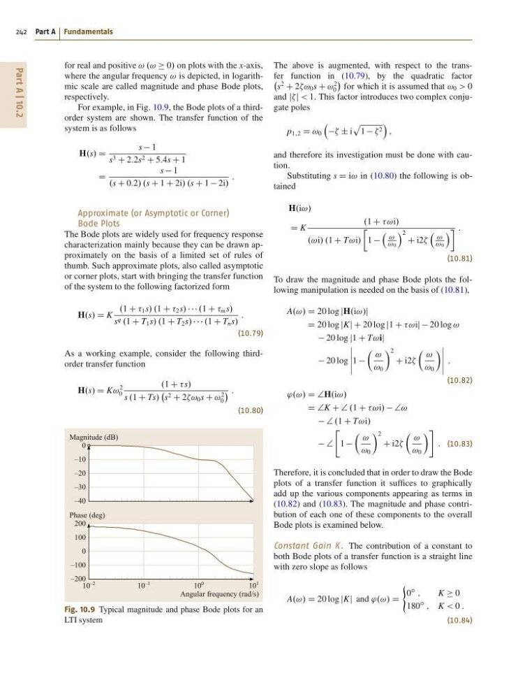
For example, in Fig. 10.9, the Bode plots of a thirdorder system are shown. The transfer function of the
system is as follows
H.s/ D
s 1
s 3 C 2:2s 2 C 5:4s C 1
D
s 1
.s C 0:2/ .s C 1 C 2i/ .s C 1 2i/
:
Approximate (or Asymptotic or Corner)
Bode Plots
The Bode plots are widely used for frequency response
characterization mainly because they can be drawn approximately on the basis of a limited set of rules of
thumb. Such approximate plots, also called asymptotic
or corner plots, start with bringing the transfer function
of the system to the following factorized form
H.s/ D K
.1 C 1 s/ .1 C 2 s/ .1 C m s/
s q .1 C T 1 s/ .1 C T 2 s/ .1 C T n s/
:
(10.79)
As a working example, consider the following thirdorder transfer function
H.s/ D K!
2
0
.1 C s/
s .1 C Ts/
s 2 C 2! 0 s C !
2
0
:
(10.80)
Magnitude (dB)
0
–10
–20
–30
–40
10
–2
10
–1
10
0
10
1
Phase (deg)
Angular frequency (rad/s)
200
100
0
–100
–200
Fig. 10.9 Typical magnitude and phase Bode plots for an
LTI system
The above is augmented, with respect to the transfer function in (10.79), by the quadratic factor
s
2
C 2! 0 s C !
2
0
for which it is assumed that ! 0 > 0
and jj < 1. This factor introduces two complex conjugate poles
p 1;2 D ! 0
˙ i
p
1 2
Á
;
and therefore its investigation must be done with caution.
Substituting s D i! in (10.80) the following is obtained
H.i!/
D K
.1 C !i/
.!i/ .1 C T!i/
Ä
1
!
!0
Á 2 C i2
!
!0
Á :
(10.81)
To draw the magnitude and phase Bode plots the following manipulation is needed on the basis of (10.81),
A.!/ D 20 log jH.i!/j
D 20 log jKj C 20 log j1 C !ij 20 log !
20 log j1 C T!ij
20 log
ˇ
ˇ
ˇ
ˇ
ˇ
1
 !
! 0
à 2
C i2
 !
! 0
à ˇ
ˇ
ˇ
ˇ
ˇ
:
(10.82)
'.!/ D †H.i!/
D †K C † .1 C !i/ †!
† .1 C T!i/
†
"
1
 !
! 0
à 2
C i2
 !
! 0
à #
: (10.83)
Therefore, it is concluded that in order to draw the Bode
plots of a transfer function it suffices to graphically
add up the various components appearing as terms in
(10.82) and (10.83). The magnitude and phase contribution of each one of these components to the overall
Bode plots is examined below.
Constant Gain K. The contribution of a constant to
both Bode plots of a transfer function is a straight line
with zero slope as follows
A.!/ D 20 log jKj and '.!/ D
(
0
ı
;
K 0
180
ı
; K < 0 :
(10.84)
242 Part A Fundamentals
for real and positive ! .! 0/ on plots with the x-axis,
where the angular frequency ! is depicted, in logarithmic scale are called magnitude and phase Bode plots,
respectively.
For example, in Fig. 10.9, the Bode plots of a thirdorder system are shown. The transfer function of the
system is as follows
H.s/ D
s 1
s 3 C 2:2s 2 C 5:4s C 1
D
s 1
.s C 0:2/ .s C 1 C 2i/ .s C 1 2i/
:
Approximate (or Asymptotic or Corner)
Bode Plots
The Bode plots are widely used for frequency response
characterization mainly because they can be drawn approximately on the basis of a limited set of rules of
thumb. Such approximate plots, also called asymptotic
or corner plots, start with bringing the transfer function
of the system to the following factorized form
H.s/ D K
.1 C 1 s/ .1 C 2 s/ .1 C m s/
s q .1 C T 1 s/ .1 C T 2 s/ .1 C T n s/
:
(10.79)
As a working example, consider the following thirdorder transfer function
H.s/ D K!
2
0
.1 C s/
s .1 C Ts/
s 2 C 2! 0 s C !
2
0
:
(10.80)
Magnitude (dB)
0
–10
–20
–30
–40
10
–2
10
–1
10
0
10
1
Phase (deg)
Angular frequency (rad/s)
200
100
0
–100
–200
Fig. 10.9 Typical magnitude and phase Bode plots for an
LTI system
The above is augmented, with respect to the transfer function in (10.79), by the quadratic factor
s
2
C 2! 0 s C !
2
0
for which it is assumed that ! 0 > 0
and jj < 1. This factor introduces two complex conjugate poles
p 1;2 D ! 0
˙ i
p
1 2
Á
;
and therefore its investigation must be done with caution.
Substituting s D i! in (10.80) the following is obtained
H.i!/
D K
.1 C !i/
.!i/ .1 C T!i/
Ä
1
!
!0
Á 2 C i2
!
!0
Á :
(10.81)
To draw the magnitude and phase Bode plots the following manipulation is needed on the basis of (10.81),
A.!/ D 20 log jH.i!/j
D 20 log jKj C 20 log j1 C !ij 20 log !
20 log j1 C T!ij
20 log
ˇ
ˇ
ˇ
ˇ
ˇ
1
 !
! 0
à 2
C i2
 !
! 0
à ˇ
ˇ
ˇ
ˇ
ˇ
:
(10.82)
'.!/ D †H.i!/
D †K C † .1 C !i/ †!
† .1 C T!i/
†
"
1
 !
! 0
à 2
C i2
 !
! 0
à #
: (10.83)
Therefore, it is concluded that in order to draw the Bode
plots of a transfer function it suffices to graphically
add up the various components appearing as terms in
(10.82) and (10.83). The magnitude and phase contribution of each one of these components to the overall
Bode plots is examined below.
Constant Gain K. The contribution of a constant to
both Bode plots of a transfer function is a straight line
with zero slope as follows
A.!/ D 20 log jKj and '.!/ D
(
0
ı
;
K 0
180
ı
; K < 0 :
(10.84)