

Control Theory and Applications 10.2 Analysis of LTI Systems 241
Part A | 10.2
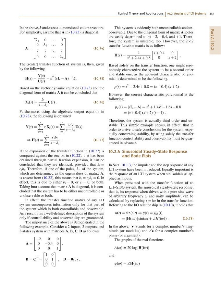
In the above, b and c are n-dimensioned column vectors.
For simplicity, assume that A in (10.73) is diagonal.
A D
2
6
6
6
4
1 0 : : : 0
0 2 : : : 0
: : :
: : :
: : :
: : :
0
0 : : : : n
3
7
7
7
5
(10.74)
The (scalar) transfer function of system is, then, given
by the following
H.s/ D
Y.s/
U.s/
D c
T
.sI n A/
1 b :
(10.75)
Based on the vector dynamic equation (10.73) and the
diagonal form of matrix A it can be concluded that
X i .s/ D
b i
s i
U.s/ :
(10.76)
Furthermore, using the algebraic output equation in
(10.73), the following is obtained
Y.s/ D
n
X
iD1
c i X i .s/ D
n
X
iD1
c i b i
s i
U.s/
) H.s/ D
n
X
iD1
c i b i
s i
:
(10.77)
If the expansion of the transfer function in (10.77) is
compared against the one on in (10.22), that has been
obtained through partial fraction expansion, it can be
concluded that they are identical, provided that k i Á
c i b i . Therefore, if one of the poles, i , of the system,
which are determined as the eigenvalues of matrix A,
is absent from (10.22), this means that k i Á c i b i D 0. In
effect, this is due to either b i D 0, or c i D 0, or both.
Taking into account that matrix A is diagonal, it is concluded that the system has to be either uncontrollable or
unobservable or both.
In effect, the transfer function matrix of any LTI
system encompasses information only for that part of
the system which is both controllable and observable.
As a result, it is a well-defined description of the system
only if controllability and observability are guaranteed.
The importance of the above is demonstrated in the
following example. Consider a 2-inputs, 2-outputs, and
3-states system with matrices A, B, C, D as follows
A D
2
4
2
0
0
0 0:4 0
0
0
1
3
5 ;
B D C
T
D
2
4
1 0
0 1
0 0
3
5 ; D D 0 22 :
This system is evidently both uncontrollable and unobservable. Due to the diagonal form of matrix A, poles
are easily determined to be 2, 0:4, and C1. Therefore, the system is unstable, too. However, the 2 2
transfer function matrix is as follows
H.s/ D
1
s 2 C 2:4s C 0:8
Ä
s C 0:4
0
0
s C 2
:
Based solely on the transfer function, one might erroneously characterize the system to be a second order
and stable one, as the apparent characteristic polynomial is determined to be the following,
p.s/ D s
2
C 2:4s C 0:8 D .s C 0:4/ .s C 2/ :
However, the correct characteristic polynomial is the
following,
p c .s/ D jsI n Aj D s
3
C 1:4s
2
1:6s 0:8
D .s C 0:4/ .s C 2/ .s 1/ :
Therefore, the system is actually third order and unstable. This simple example shows, in effect, that in
order to arrive to safe conclusions for the system, especially concerning stability, by using solely the transfer
function controllability and observability must be guaranteed in advance.
10.2.4 Sinusoidal Steady-State Response
and Bode Plots
In Sect. 10.1.3, the impulse and the step response of any
LTI system have been introduced. Equally important is
the response of an LTI system when sinusoidals as applied as inputs.
When presented with the transfer function of an
LTI–SISO system, the sinusoidal steady-state response,
that is, its response when driven with a pure sine wave
of arbitrary frequency ! and unity amplitude, can be
calculated by replacing s D i! in the transfer function.
Referring to the I/O relationship in (10.10), it holds that
u.t/ D sin.!t/ ) y.t/ D y SS .t/
D jH.i!/j sin.!t C †H.i!// :
(10.78)
In the above, jj stands for a complex number’s magnitude (or modulus) and †† for a complex number’s
phase (or argument).
The graphs of the real functions
A.!/ D 20 log jH.i!/j
and
'.!/ D †H.i!/
Part A | 10.2
In the above, b and c are n-dimensioned column vectors.
For simplicity, assume that A in (10.73) is diagonal.
A D
2
6
6
6
4
1 0 : : : 0
0 2 : : : 0
: : :
: : :
: : :
: : :
0
0 : : : : n
3
7
7
7
5
(10.74)
The (scalar) transfer function of system is, then, given
by the following
H.s/ D
Y.s/
U.s/
D c
T
.sI n A/
1 b :
(10.75)
Based on the vector dynamic equation (10.73) and the
diagonal form of matrix A it can be concluded that
X i .s/ D
b i
s i
U.s/ :
(10.76)
Furthermore, using the algebraic output equation in
(10.73), the following is obtained
Y.s/ D
n
X
iD1
c i X i .s/ D
n
X
iD1
c i b i
s i
U.s/
) H.s/ D
n
X
iD1
c i b i
s i
:
(10.77)
If the expansion of the transfer function in (10.77) is
compared against the one on in (10.22), that has been
obtained through partial fraction expansion, it can be
concluded that they are identical, provided that k i Á
c i b i . Therefore, if one of the poles, i , of the system,
which are determined as the eigenvalues of matrix A,
is absent from (10.22), this means that k i Á c i b i D 0. In
effect, this is due to either b i D 0, or c i D 0, or both.
Taking into account that matrix A is diagonal, it is concluded that the system has to be either uncontrollable or
unobservable or both.
In effect, the transfer function matrix of any LTI
system encompasses information only for that part of
the system which is both controllable and observable.
As a result, it is a well-defined description of the system
only if controllability and observability are guaranteed.
The importance of the above is demonstrated in the
following example. Consider a 2-inputs, 2-outputs, and
3-states system with matrices A, B, C, D as follows
A D
2
4
2
0
0
0 0:4 0
0
0
1
3
5 ;
B D C
T
D
2
4
1 0
0 1
0 0
3
5 ; D D 0 22 :
This system is evidently both uncontrollable and unobservable. Due to the diagonal form of matrix A, poles
are easily determined to be 2, 0:4, and C1. Therefore, the system is unstable, too. However, the 2 2
transfer function matrix is as follows
H.s/ D
1
s 2 C 2:4s C 0:8
Ä
s C 0:4
0
0
s C 2
:
Based solely on the transfer function, one might erroneously characterize the system to be a second order
and stable one, as the apparent characteristic polynomial is determined to be the following,
p.s/ D s
2
C 2:4s C 0:8 D .s C 0:4/ .s C 2/ :
However, the correct characteristic polynomial is the
following,
p c .s/ D jsI n Aj D s
3
C 1:4s
2
1:6s 0:8
D .s C 0:4/ .s C 2/ .s 1/ :
Therefore, the system is actually third order and unstable. This simple example shows, in effect, that in
order to arrive to safe conclusions for the system, especially concerning stability, by using solely the transfer
function controllability and observability must be guaranteed in advance.
10.2.4 Sinusoidal Steady-State Response
and Bode Plots
In Sect. 10.1.3, the impulse and the step response of any
LTI system have been introduced. Equally important is
the response of an LTI system when sinusoidals as applied as inputs.
When presented with the transfer function of an
LTI–SISO system, the sinusoidal steady-state response,
that is, its response when driven with a pure sine wave
of arbitrary frequency ! and unity amplitude, can be
calculated by replacing s D i! in the transfer function.
Referring to the I/O relationship in (10.10), it holds that
u.t/ D sin.!t/ ) y.t/ D y SS .t/
D jH.i!/j sin.!t C †H.i!// :
(10.78)
In the above, jj stands for a complex number’s magnitude (or modulus) and †† for a complex number’s
phase (or argument).
The graphs of the real functions
A.!/ D 20 log jH.i!/j
and
'.!/ D †H.i!/