

Part A | 10.2
238 Part A Fundamentals
Output signal
y
H 1 (s)
Input signal
u
1
s + 1
H 2 (s)
s + 2
s
2 + s + 1
1
s
2 + 5s + 4
H 3 (s)
Fig. 10.4 Cascade interconnection of
scalar transfer functions
Output signal
....
Input signals
Fig. 10.5 Summing junction used in block diagrams
Direct branch
Feedback branch
r
u
y
F (s)
G (s)
Fig. 10.6 Block diagram of a typical closed-loop system
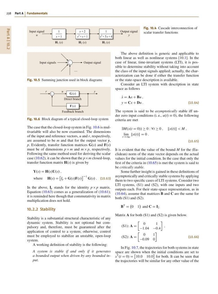
The case that the closed-loop system in Fig. 10.6 is multivariable will also be now examined. The dimensions
of the input and reference vectors, u and r, respectively,
are assumed to be m and that for the output vector y,
p. Evidently, transfer function matrices G.s/ and F.s/
must be of dimensions p m and m p, respectively.
Following the same method used for deriving the scalar
case (10.62), it can be shown that the p m closed-loop,
transfer function matrix H.s/ is given by
Y.s/ D H.s/U.s/ ;
where H.s/ D
I p C G.s/F.s/
1 G.s/ : (10.63)
In the above, I p stands for the identity p p matrix.
Equation (10.63) comes as a generalization of (10.61);
it is reminded here though that commutativity in matrix
multiplication does not hold.
10.2.2 Stability
Stability is a substantial structural characteristic of any
dynamic system. Stability is not optional but compulsory and, therefore, must be guaranteed after the
application of control to a system; otherwise, control
must be employed to stabilize an unstable, open-loop
system.
A working definition of stability is the following:
A system is stable if and only if it generates
a bounded output when driven by any bounded input.
The above definition is generic and applicable to
both linear as well as nonlinear systems [10.1]. In the
case of linear, time-invariant systems (LTI), it is possible to determine stability without taking into account
the class of the input signals applied; actually, the characterization can be done if either the transfer function
or the state-space description is available.
Consider an LTI system with description in state
space as follows
P
x D Ax C Bu ;
y D Cx C Du :
(10.64)
The system is said to be asymptotically stable iff under zero input conditions (i. e., u.t/ Á 0), the following
criteria are met
9M.x.t D 0// 0 W 8t 0 ; kx.t/k < M ;
lim
t!1
kx.t/k D 0 :
(10.65)
It is evident that the value of the bound M for the (Euclidean) norm of the state vector depends on the actual
values for the initial condition. In the case that only the
first of the criteria in (10.65) is met the system is said to
be critically stable.
Some further insight is gained in these definitions of
asymptotically and critically stable systems by applying
them to two specific cases of LTI systems. Consider two
LTI systems, (S1) and (S2), with one inputs and two
outputs each. For their state-space representation, as in
(10.64), assume that matrices B and C are the same for
both (S1) and (S2).
B
T
D
0 1
and C D I 2
Matrix A for both (S1) and (S2) is given below.
(S1): A D
Ä
0
1
1:04 0:4
;
(S2): A D
Ä
0
1
0:09 0
(10.66)
In Fig. 10.7, the trajectories for both systems in state
space are shown when the initial conditions are set to
x
T
.t D 0/ D
10:0 10:0
for both. It can be seen that
the trajectories will be similar for any other value of the
238 Part A Fundamentals
Output signal
y
H 1 (s)
Input signal
u
1
s + 1
H 2 (s)
s + 2
s
2 + s + 1
1
s
2 + 5s + 4
H 3 (s)
Fig. 10.4 Cascade interconnection of
scalar transfer functions
Output signal
....
Input signals
Fig. 10.5 Summing junction used in block diagrams
Direct branch
Feedback branch
r
u
y
F (s)
G (s)
Fig. 10.6 Block diagram of a typical closed-loop system
The case that the closed-loop system in Fig. 10.6 is multivariable will also be now examined. The dimensions
of the input and reference vectors, u and r, respectively,
are assumed to be m and that for the output vector y,
p. Evidently, transfer function matrices G.s/ and F.s/
must be of dimensions p m and m p, respectively.
Following the same method used for deriving the scalar
case (10.62), it can be shown that the p m closed-loop,
transfer function matrix H.s/ is given by
Y.s/ D H.s/U.s/ ;
where H.s/ D
I p C G.s/F.s/
1 G.s/ : (10.63)
In the above, I p stands for the identity p p matrix.
Equation (10.63) comes as a generalization of (10.61);
it is reminded here though that commutativity in matrix
multiplication does not hold.
10.2.2 Stability
Stability is a substantial structural characteristic of any
dynamic system. Stability is not optional but compulsory and, therefore, must be guaranteed after the
application of control to a system; otherwise, control
must be employed to stabilize an unstable, open-loop
system.
A working definition of stability is the following:
A system is stable if and only if it generates
a bounded output when driven by any bounded input.
The above definition is generic and applicable to
both linear as well as nonlinear systems [10.1]. In the
case of linear, time-invariant systems (LTI), it is possible to determine stability without taking into account
the class of the input signals applied; actually, the characterization can be done if either the transfer function
or the state-space description is available.
Consider an LTI system with description in state
space as follows
P
x D Ax C Bu ;
y D Cx C Du :
(10.64)
The system is said to be asymptotically stable iff under zero input conditions (i. e., u.t/ Á 0), the following
criteria are met
9M.x.t D 0// 0 W 8t 0 ; kx.t/k < M ;
lim
t!1
kx.t/k D 0 :
(10.65)
It is evident that the value of the bound M for the (Euclidean) norm of the state vector depends on the actual
values for the initial condition. In the case that only the
first of the criteria in (10.65) is met the system is said to
be critically stable.
Some further insight is gained in these definitions of
asymptotically and critically stable systems by applying
them to two specific cases of LTI systems. Consider two
LTI systems, (S1) and (S2), with one inputs and two
outputs each. For their state-space representation, as in
(10.64), assume that matrices B and C are the same for
both (S1) and (S2).
B
T
D
0 1
and C D I 2
Matrix A for both (S1) and (S2) is given below.
(S1): A D
Ä
0
1
1:04 0:4
;
(S2): A D
Ä
0
1
0:09 0
(10.66)
In Fig. 10.7, the trajectories for both systems in state
space are shown when the initial conditions are set to
x
T
.t D 0/ D
10:0 10:0
for both. It can be seen that
the trajectories will be similar for any other value of the