

Control Theory and Applications 10.2 Analysis of LTI Systems 239
Part A | 10.2
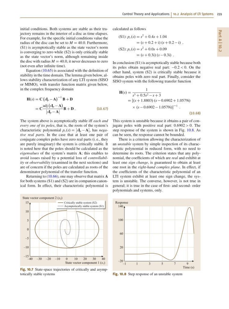
initial conditions. Both systems are stable as their trajectory remains in the interior of a disc as time elapses.
For example, for the specific initial conditions value the
radius of the disc can be set to M D 40:0. Furthermore,
(S1) is asymptotically stable as the state vector’s norm
is converging to zero while (S2) is only critically stable
as the state vector’s norm, although remaining inside
the disc with radius M D 40:0, it never decreases to zero
(not even after infinite time).
Equation (10.65) is associated with the definition of
stability in the time domain. The lemma given below, allows stability characterization of any LTI system (SISO
or MIMO), with transfer function matrix given below,
in the complex frequency domain
H.s/ D C
sI p A
1 B C D
D C
adj
sI p A
ˇ
ˇ sI p A
ˇ
ˇ
B C D :
(10.67)
The system above is asymptotically stable iff each and
every one of its poles, that is, the roots of the system’s
characteristic polynomial p c .s/ D
ˇ
ˇ sI p A
ˇ
ˇ , has negative real parts. In the case that at least one pair of
conjugate complex poles have zero real parts (i. e., they
are purely imaginary) the system is critically stable. It
is noted here that the poles should be calculated as the
eigenvalues of the system’s matrix A; this enables to
avoid issues raised by a potential loss of controllability or observability (examined in the next sections) and
are of concern if the poles are calculated as roots of the
denominator polynomial of the transfer function.
Returning to (10.66), one may observe that matrix A
for both systems (S1) and (S2) are in companion canonical form. In effect, their characteristic polynomial is
Critically stable system (S2)
Asymptotically stable system (S1)
–40 –30 –20 –10
0
10
20
30
40
State vector component 2 (x 2 )
State vector component 1 (x 1 )
15
10
5
0
–5
–10
–15
Fig. 10.7 State-space trajectories of critically and asymptotically stable systems
calculated as follows
(S1): p c .s/ D s
2
C 0:4s C 1:04
D .s C 0:2 C i/ .s C 0:2 i/ ;
(S2): p c .s/ D s
2
C 0:0s C 0:09
D .s C 0:3i/ .s 0:3i/ :
In conclusion (S1) is asymptotically stable because both
its poles obtain negative real part: 0:2 < 0. On the
other hand, system (S2) is critically stable because it
obtains poles with zero real part. Finally, consider the
SISO system with the following transfer function
H.s/ D
1
s 3 C 0:5s 2 s C 3
D Œ.s C 1:8803/ .s 0:6902 C 1:0579i/
.s 0:6902 1:0579i/
1 :
(10.68)
This system is unstable because it obtains a pair of conjugate poles with positive real part: 0:6902 > 0. The
step response of the system is shown in Fig. 10.8. As
can be seen, the response cannot be bounded.
There is a criterion allowing the characterization of
an unstable system by simple inspection of its characteristic polynomial in reduced form, with no need to
determine its roots. The criterion states that any polynomial, the coefficients of which are real and exhibit at
least one sign change, is guaranteed to obtain at least
one root in the right-hand complex plane. In effect, if
the coefficients of the characteristic polynomial of an
LTI system exhibit at least one sign change, the system is unstable. The converse, however, is not true in
general; it is true in the case of first- and second- order
polynomials and systems, only.
– 1
1
3
5
7
9
Response
Time (s)
140
100
60
20
–20
Fig. 10.8 Step response of an unstable system
Part A | 10.2
initial conditions. Both systems are stable as their trajectory remains in the interior of a disc as time elapses.
For example, for the specific initial conditions value the
radius of the disc can be set to M D 40:0. Furthermore,
(S1) is asymptotically stable as the state vector’s norm
is converging to zero while (S2) is only critically stable
as the state vector’s norm, although remaining inside
the disc with radius M D 40:0, it never decreases to zero
(not even after infinite time).
Equation (10.65) is associated with the definition of
stability in the time domain. The lemma given below, allows stability characterization of any LTI system (SISO
or MIMO), with transfer function matrix given below,
in the complex frequency domain
H.s/ D C
sI p A
1 B C D
D C
adj
sI p A
ˇ
ˇ sI p A
ˇ
ˇ
B C D :
(10.67)
The system above is asymptotically stable iff each and
every one of its poles, that is, the roots of the system’s
characteristic polynomial p c .s/ D
ˇ
ˇ sI p A
ˇ
ˇ , has negative real parts. In the case that at least one pair of
conjugate complex poles have zero real parts (i. e., they
are purely imaginary) the system is critically stable. It
is noted here that the poles should be calculated as the
eigenvalues of the system’s matrix A; this enables to
avoid issues raised by a potential loss of controllability or observability (examined in the next sections) and
are of concern if the poles are calculated as roots of the
denominator polynomial of the transfer function.
Returning to (10.66), one may observe that matrix A
for both systems (S1) and (S2) are in companion canonical form. In effect, their characteristic polynomial is
Critically stable system (S2)
Asymptotically stable system (S1)
–40 –30 –20 –10
0
10
20
30
40
State vector component 2 (x 2 )
State vector component 1 (x 1 )
15
10
5
0
–5
–10
–15
Fig. 10.7 State-space trajectories of critically and asymptotically stable systems
calculated as follows
(S1): p c .s/ D s
2
C 0:4s C 1:04
D .s C 0:2 C i/ .s C 0:2 i/ ;
(S2): p c .s/ D s
2
C 0:0s C 0:09
D .s C 0:3i/ .s 0:3i/ :
In conclusion (S1) is asymptotically stable because both
its poles obtain negative real part: 0:2 < 0. On the
other hand, system (S2) is critically stable because it
obtains poles with zero real part. Finally, consider the
SISO system with the following transfer function
H.s/ D
1
s 3 C 0:5s 2 s C 3
D Œ.s C 1:8803/ .s 0:6902 C 1:0579i/
.s 0:6902 1:0579i/
1 :
(10.68)
This system is unstable because it obtains a pair of conjugate poles with positive real part: 0:6902 > 0. The
step response of the system is shown in Fig. 10.8. As
can be seen, the response cannot be bounded.
There is a criterion allowing the characterization of
an unstable system by simple inspection of its characteristic polynomial in reduced form, with no need to
determine its roots. The criterion states that any polynomial, the coefficients of which are real and exhibit at
least one sign change, is guaranteed to obtain at least
one root in the right-hand complex plane. In effect, if
the coefficients of the characteristic polynomial of an
LTI system exhibit at least one sign change, the system is unstable. The converse, however, is not true in
general; it is true in the case of first- and second- order
polynomials and systems, only.
– 1
1
3
5
7
9
Response
Time (s)
140
100
60
20
–20
Fig. 10.8 Step response of an unstable system