

Part A | 9.5
220 Part A Fundamentals
R x;y .t/ D h .t/ ˝ R x;x
, S x;y .!/ D H
.!/ S x;x .!/ :
(9.106)
All of the above can be derived on the basis of the definitions and properties given previously, as well as the
commutativity and associativity of scalar convolution.
For example, in the case of (9.104)
R y;y .t/ D y ˝ y (t)
D Œh ˝ x ˝ Œh .t/ ˝ x .t/
D R h;h ˝ R x;x :
(9.107)
It is noted here that:
1.
S h;h .!/ D H.!/H
.!/ D jH.!/j
2
;
2.
R h;h ../ D
C1 Z
1
S h;h .f /e
i!! df
D
C1 Z
1
jH.!/j
2 e
i!! df ; ! D 2f ;
and
3.
0
@
x (t)
y (t)
h (t)
1
A .t/ D
0
@
x
y
h
1
A .t/; 8t 2 R , F
8
<
:
x (t)
y (t)
h (t)
.t/
9
=
;
D
0
@
X
Y
H
1
A .! or f / :
9.5 Optimal Signal Estimation
9.5.1 System Identification
One of the most fundamental problems in science and
engineering is the determination of a system’s dynamics, preferably in the form of a mathematical model,
when presented with the system response(s) to given
deterministic or random driving inputs. This is the fundamental system identification problem [9.7, 8].
In the case of an LTI system, especially in the
case of discrete-time or sampled-data systems, system identification is essentially equivalent to a problem
of minimum square error approximation. Consider the
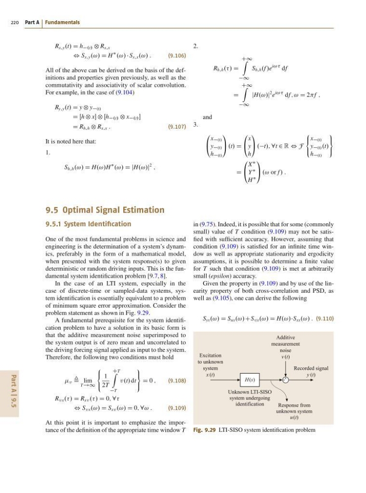
problem statement as shown in Fig. 9.29.
A fundamental prerequisite for the system identification problem to have a solution in its basic form is
that the additive measurement noise superimposed to
the system output is of zero mean and uncorrelated to
the driving forcing signal applied as input to the system.
Therefore, the following two conditions must hold
v , lim
T!1
8
<
:
1
2T
CT
Z
T
v .t/ dt
9
=
;
D 0 ;
(9.108)
R v x ../ D R xv ../ D 0; 8
, S v x .!/ D S xv .!/ D 0; 8! :
(9.109)
At this point it is important to emphasize the importance of the definition of the appropriate time window T
in (9.75). Indeed, it is possible that for some (commonly
small) value of T condition (9.109) may not be satisfied with sufficient accuracy. However, assuming that
condition (9.109) is satisfied for an infinite time window as well as appropriate stationarity and ergodicity
assumptions, it is possible to determine a finite value
for T such that condition (9.109) is met at arbitrarily
small (epsilon) accuracy.
Given the property in (9.109) and by use of the linearity property of both cross-correlation and PSD, as
well as (9.105), one can derive the following
S yx .!/ D S ux .!/CS v x .!/ D H.!/S xx .!/ : (9.110)
H (s)
Unknown LTI-SISO
system undergoing
identification
Response from
unknown system
u (t)
Recorded signal
y (t)
Excitation
to unknown
system
x (t)
Additive
measurement
noise
v (t)
Fig. 9.29 LTI-SISO system identification problem
220 Part A Fundamentals
R x;y .t/ D h .t/ ˝ R x;x
, S x;y .!/ D H
.!/ S x;x .!/ :
(9.106)
All of the above can be derived on the basis of the definitions and properties given previously, as well as the
commutativity and associativity of scalar convolution.
For example, in the case of (9.104)
R y;y .t/ D y ˝ y (t)
D Œh ˝ x ˝ Œh .t/ ˝ x .t/
D R h;h ˝ R x;x :
(9.107)
It is noted here that:
1.
S h;h .!/ D H.!/H
.!/ D jH.!/j
2
;
2.
R h;h ../ D
C1 Z
1
S h;h .f /e
i!! df
D
C1 Z
1
jH.!/j
2 e
i!! df ; ! D 2f ;
and
3.
0
@
x (t)
y (t)
h (t)
1
A .t/ D
0
@
x
y
h
1
A .t/; 8t 2 R , F
8
<
:
x (t)
y (t)
h (t)
.t/
9
=
;
D
0
@
X
Y
H
1
A .! or f / :
9.5 Optimal Signal Estimation
9.5.1 System Identification
One of the most fundamental problems in science and
engineering is the determination of a system’s dynamics, preferably in the form of a mathematical model,
when presented with the system response(s) to given
deterministic or random driving inputs. This is the fundamental system identification problem [9.7, 8].
In the case of an LTI system, especially in the
case of discrete-time or sampled-data systems, system identification is essentially equivalent to a problem
of minimum square error approximation. Consider the
problem statement as shown in Fig. 9.29.
A fundamental prerequisite for the system identification problem to have a solution in its basic form is
that the additive measurement noise superimposed to
the system output is of zero mean and uncorrelated to
the driving forcing signal applied as input to the system.
Therefore, the following two conditions must hold
v , lim
T!1
8
<
:
1
2T
CT
Z
T
v .t/ dt
9
=
;
D 0 ;
(9.108)
R v x ../ D R xv ../ D 0; 8
, S v x .!/ D S xv .!/ D 0; 8! :
(9.109)
At this point it is important to emphasize the importance of the definition of the appropriate time window T
in (9.75). Indeed, it is possible that for some (commonly
small) value of T condition (9.109) may not be satisfied with sufficient accuracy. However, assuming that
condition (9.109) is satisfied for an infinite time window as well as appropriate stationarity and ergodicity
assumptions, it is possible to determine a finite value
for T such that condition (9.109) is met at arbitrarily
small (epsilon) accuracy.
Given the property in (9.109) and by use of the linearity property of both cross-correlation and PSD, as
well as (9.105), one can derive the following
S yx .!/ D S ux .!/CS v x .!/ D H.!/S xx .!/ : (9.110)
H (s)
Unknown LTI-SISO
system undergoing
identification
Response from
unknown system
u (t)
Recorded signal
y (t)
Excitation
to unknown
system
x (t)
Additive
measurement
noise
v (t)
Fig. 9.29 LTI-SISO system identification problem