

Digital Signal Processing 9.4 Waveform Analysis 219
Part A | 9.4
In effect, the PSD of a single signal is an even, nonnegative complex function of frequency. Also, for the
autocorrelation it holds that it is an even function of
time , i. e., R x;x ../ D R x;x ./.
A final note has to do with the extension of the
PSD concept to random signals (stochastic processes in
mathematical terminology). Assuming ergodicity and
WSS, the Wiener–Khinchin theorem can be employed
to introduce a PSD for a random signal X or at least
a power spectral distribution function F X .f / as follows
hX.t/; X.t C /i D R X;X ../
D
C1 Z
1
e
i!! dF X .f /; ! D 2f :
(9.98)
For the above to hold, the autocorrelation of X needs to
exist and be finite for any value of time shift variable ,
but its Fourier transform may not be well defined. Indeed, the Fourier transform of a random signal may not
exist in general, because stationary stochastic processes
may not generally be square or absolutely integrable.
Nor does their autocorrelation need to be absolutely integrable, so it need not have a Fourier transform, either.
However, in most practical applications the autocorrelation is integrable and even satisfies the conditions to
obtain a Fourier transform. In this case, the PSD can be
introduced through the Fourier transform as follows
S X;X .!/ D
C1 Z
1
R X;X ../e
i!! d , R X;X ../
D
C1 Z
1
S X;X .f /e
i!! df ; ! D 2f :
(9.99)
Finally, in this case the PSD is the averaged derivative
of the power spectral distribution function introduced
previously. This is why the latter is also referred to as
the integrated spectrum of the stochastic process.
9.4.3 Waveform Propagation Through
a Linear, Time-Invariant System
Consider a linear, time-invariant (LTI) system with
a single input and a single output (SISO), as shown in
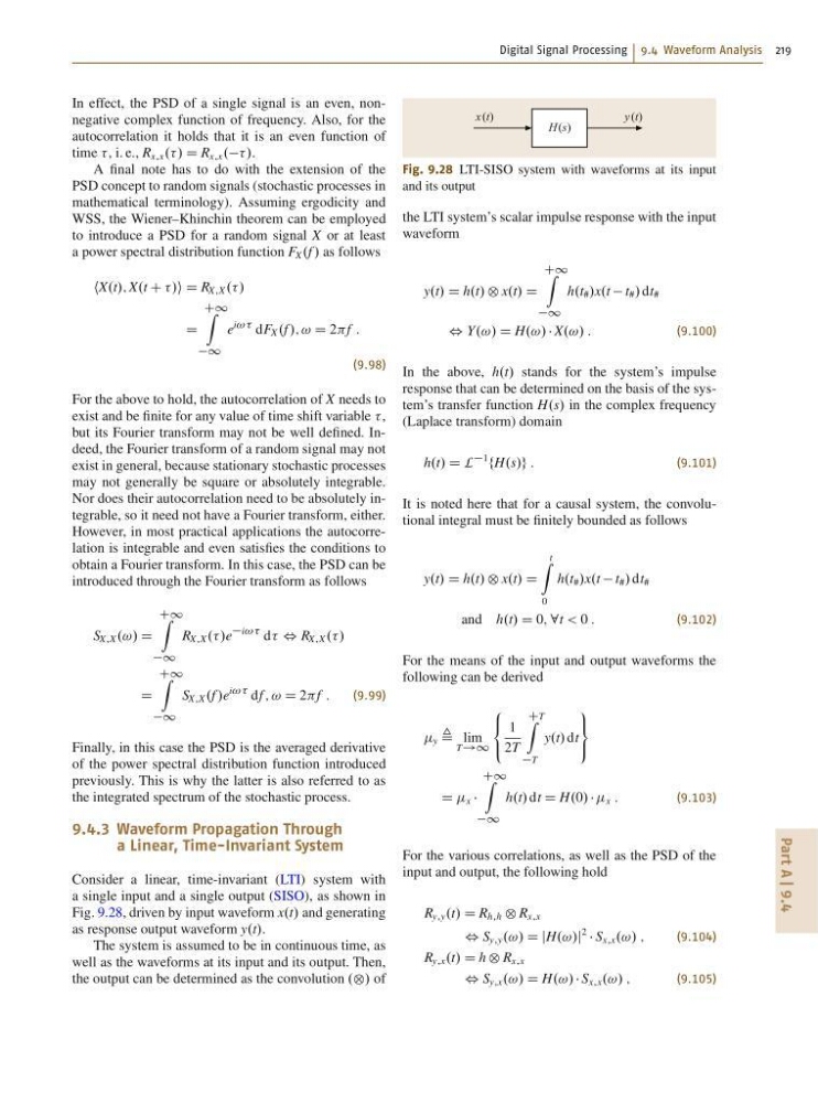
Fig. 9.28, driven by input waveform x.t/ and generating
as response output waveform y.t/.
The system is assumed to be in continuous time, as
well as the waveforms at its input and its output. Then,
the output can be determined as the convolution .˝/ of
H (s)
y (t)
x (t)
Fig. 9.28 LTI-SISO system with waveforms at its input
and its output
the LTI system’s scalar impulse response with the input
waveform
y.t/ D h.t/ ˝ x.t/ D
C1 Z
1
h.t # /x.t t # / dt #
, Y.!/ D H.!/ X.!/ :
(9.100)
In the above, h.t/ stands for the system’s impulse
response that can be determined on the basis of the system’s transfer function H.s/ in the complex frequency
(Laplace transform) domain
h.t/ D L
1
fH.s/g :
(9.101)
It is noted here that for a causal system, the convolutional integral must be finitely bounded as follows
y.t/ D h.t/ ˝ x.t/ D
t
Z
0
h.t # /x.t t # / dt #
and h.t/ D 0; 8t < 0 :
(9.102)
For the means of the input and output waveforms the
following can be derived
y , lim
T!1
8
<
:
1
2T
CT
Z
T
y.t/ dt
9
=
;
D x
C1 Z
1
h.t/ dt D H.0/ x :
(9.103)
For the various correlations, as well as the PSD of the
input and output, the following hold
R y;y .t/ D R h;h ˝ R x;x
, S y;y .!/ D jH.!/j
2
S x;x .!/ ;
(9.104)
R y;x .t/ D h ˝ R x;x
, S y;x .!/ D H.!/ S x;x .!/ ;
(9.105)
Part A | 9.4
In effect, the PSD of a single signal is an even, nonnegative complex function of frequency. Also, for the
autocorrelation it holds that it is an even function of
time , i. e., R x;x ../ D R x;x ./.
A final note has to do with the extension of the
PSD concept to random signals (stochastic processes in
mathematical terminology). Assuming ergodicity and
WSS, the Wiener–Khinchin theorem can be employed
to introduce a PSD for a random signal X or at least
a power spectral distribution function F X .f / as follows
hX.t/; X.t C /i D R X;X ../
D
C1 Z
1
e
i!! dF X .f /; ! D 2f :
(9.98)
For the above to hold, the autocorrelation of X needs to
exist and be finite for any value of time shift variable ,
but its Fourier transform may not be well defined. Indeed, the Fourier transform of a random signal may not
exist in general, because stationary stochastic processes
may not generally be square or absolutely integrable.
Nor does their autocorrelation need to be absolutely integrable, so it need not have a Fourier transform, either.
However, in most practical applications the autocorrelation is integrable and even satisfies the conditions to
obtain a Fourier transform. In this case, the PSD can be
introduced through the Fourier transform as follows
S X;X .!/ D
C1 Z
1
R X;X ../e
i!! d , R X;X ../
D
C1 Z
1
S X;X .f /e
i!! df ; ! D 2f :
(9.99)
Finally, in this case the PSD is the averaged derivative
of the power spectral distribution function introduced
previously. This is why the latter is also referred to as
the integrated spectrum of the stochastic process.
9.4.3 Waveform Propagation Through
a Linear, Time-Invariant System
Consider a linear, time-invariant (LTI) system with
a single input and a single output (SISO), as shown in
Fig. 9.28, driven by input waveform x.t/ and generating
as response output waveform y.t/.
The system is assumed to be in continuous time, as
well as the waveforms at its input and its output. Then,
the output can be determined as the convolution .˝/ of
H (s)
y (t)
x (t)
Fig. 9.28 LTI-SISO system with waveforms at its input
and its output
the LTI system’s scalar impulse response with the input
waveform
y.t/ D h.t/ ˝ x.t/ D
C1 Z
1
h.t # /x.t t # / dt #
, Y.!/ D H.!/ X.!/ :
(9.100)
In the above, h.t/ stands for the system’s impulse
response that can be determined on the basis of the system’s transfer function H.s/ in the complex frequency
(Laplace transform) domain
h.t/ D L
1
fH.s/g :
(9.101)
It is noted here that for a causal system, the convolutional integral must be finitely bounded as follows
y.t/ D h.t/ ˝ x.t/ D
t
Z
0
h.t # /x.t t # / dt #
and h.t/ D 0; 8t < 0 :
(9.102)
For the means of the input and output waveforms the
following can be derived
y , lim
T!1
8
<
:
1
2T
CT
Z
T
y.t/ dt
9
=
;
D x
C1 Z
1
h.t/ dt D H.0/ x :
(9.103)
For the various correlations, as well as the PSD of the
input and output, the following hold
R y;y .t/ D R h;h ˝ R x;x
, S y;y .!/ D jH.!/j
2
S x;x .!/ ;
(9.104)
R y;x .t/ D h ˝ R x;x
, S y;x .!/ D H.!/ S x;x .!/ ;
(9.105)