

Part A | 9.1
200 Part A Fundamentals
0
2ω max
– ω max
+ω max
|X (ω)|
Fig. 9.3 Typical spectrum of real low-pass signal
ality between multiplication and convolution, one can
determine the spectrum of signal x • .t/ at the output of
an ideal sampler
x • .t/ D x.t/
C1 X
nDD1
•.t nT s / )
) X • .!/ D X.!/ ˝ F
( C1 X
nDD1
•.t nT s /
)
D ! s X.!/ ˝
C1 X
nD0
•.! n! s /
) X • .!/ D ! s
C1 X
nD0
X.!/ ˝ •.! n! s /
D ! s
C1 X
nD0
C1 Z
1
X../•.! n! s / d :
The following property of the Dirac impulse delta can
now be employed
.r/ ˝ •.r r 0 /
D
C1 Z
1
../•.r r 0 / d D .r r 0 / :
(9.14)
Eventually one obtains
X • .!/ D F
( C1 X
nDD1
x.nT s /•.t nT s /
)
D ! s
C1 X
nD0
X.! n! s / :
(9.15)
Using (9.15) one can assess the effect of sampling
on spectrum X.!/ of the analog, the continuous-time
signal at the input. Sampling introduces, therefore, an
infinite number of aliases of spectrum X.!/ of the analog signal, centered at integer multiples of the sampling
circular frequency ! s .
To visualize this, consider a real signal with all its
spectral content lying within the low frequency range
(low-pass or baseband signal); like, e.g., the signal with
spectrum as in Fig. 9.3. Note that the amplitude spectrum jX.!/j of the signal is an odd function of circular
frequency ! due to the fact is assumed to be purely real
in the time domain.
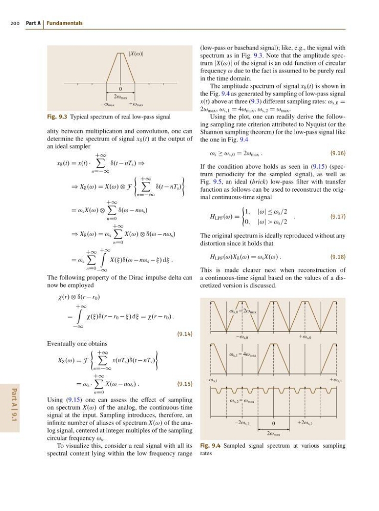
The amplitude spectrum of signal x • .t/ is shown in
the Fig. 9.4 as generated by sampling of low-pass signal
x.t/ above at three (9.3) different sampling rates: ! s;0 D
2! max , ! s;1 D 4! max , ! s;2 D ! max .
Using the plot, one can readily derive the following sampling rate criterion attributed to Nyquist (or the
Shannon sampling theorem) for the low-pass signal like
the one in Fig. 9.4
! s ! s;0 D 2! max :
(9.16)
If the condition above holds as seen in (9.15) (spectrum periodicity for the sampled signal), as well as
Fig. 9.5, an ideal (brick) low-pass filter with transfer
function as follows can be used to reconstruct the original continuous-time signal
H LPF .!/ D
(
1; j!j Ä ! s =2
0; j!j > ! s =2
:
(9.17)
The original spectrum is ideally reproduced without any
distortion since it holds that
H LPF .!/X • .!/ D ! s X.!/ :
(9.18)
This is made clearer next when reconstruction of
a continuous-time signal based on the values of a discretized version is discussed.
– ω s,1
– ω s,0
+ω s,0
+ω s,1
ω s,1 = 4ω max
ω s,0 = 2ω max
0
–2ω s,2
2ω max
+2ω s,2
ω s,2 = ω max
Fig. 9.4 Sampled signal spectrum at various sampling
rates
200 Part A Fundamentals
0
2ω max
– ω max
+ω max
|X (ω)|
Fig. 9.3 Typical spectrum of real low-pass signal
ality between multiplication and convolution, one can
determine the spectrum of signal x • .t/ at the output of
an ideal sampler
x • .t/ D x.t/
C1 X
nDD1
•.t nT s / )
) X • .!/ D X.!/ ˝ F
( C1 X
nDD1
•.t nT s /
)
D ! s X.!/ ˝
C1 X
nD0
•.! n! s /
) X • .!/ D ! s
C1 X
nD0
X.!/ ˝ •.! n! s /
D ! s
C1 X
nD0
C1 Z
1
X../•.! n! s / d :
The following property of the Dirac impulse delta can
now be employed
.r/ ˝ •.r r 0 /
D
C1 Z
1
../•.r r 0 / d D .r r 0 / :
(9.14)
Eventually one obtains
X • .!/ D F
( C1 X
nDD1
x.nT s /•.t nT s /
)
D ! s
C1 X
nD0
X.! n! s / :
(9.15)
Using (9.15) one can assess the effect of sampling
on spectrum X.!/ of the analog, the continuous-time
signal at the input. Sampling introduces, therefore, an
infinite number of aliases of spectrum X.!/ of the analog signal, centered at integer multiples of the sampling
circular frequency ! s .
To visualize this, consider a real signal with all its
spectral content lying within the low frequency range
(low-pass or baseband signal); like, e.g., the signal with
spectrum as in Fig. 9.3. Note that the amplitude spectrum jX.!/j of the signal is an odd function of circular
frequency ! due to the fact is assumed to be purely real
in the time domain.
The amplitude spectrum of signal x • .t/ is shown in
the Fig. 9.4 as generated by sampling of low-pass signal
x.t/ above at three (9.3) different sampling rates: ! s;0 D
2! max , ! s;1 D 4! max , ! s;2 D ! max .
Using the plot, one can readily derive the following sampling rate criterion attributed to Nyquist (or the
Shannon sampling theorem) for the low-pass signal like
the one in Fig. 9.4
! s ! s;0 D 2! max :
(9.16)
If the condition above holds as seen in (9.15) (spectrum periodicity for the sampled signal), as well as
Fig. 9.5, an ideal (brick) low-pass filter with transfer
function as follows can be used to reconstruct the original continuous-time signal
H LPF .!/ D
(
1; j!j Ä ! s =2
0; j!j > ! s =2
:
(9.17)
The original spectrum is ideally reproduced without any
distortion since it holds that
H LPF .!/X • .!/ D ! s X.!/ :
(9.18)
This is made clearer next when reconstruction of
a continuous-time signal based on the values of a discretized version is discussed.
– ω s,1
– ω s,0
+ω s,0
+ω s,1
ω s,1 = 4ω max
ω s,0 = 2ω max
0
–2ω s,2
2ω max
+2ω s,2
ω s,2 = ω max
Fig. 9.4 Sampled signal spectrum at various sampling
rates