

Digital Signal Processing 9.1 Discrete-Time Systems 199
Part A | 9.1
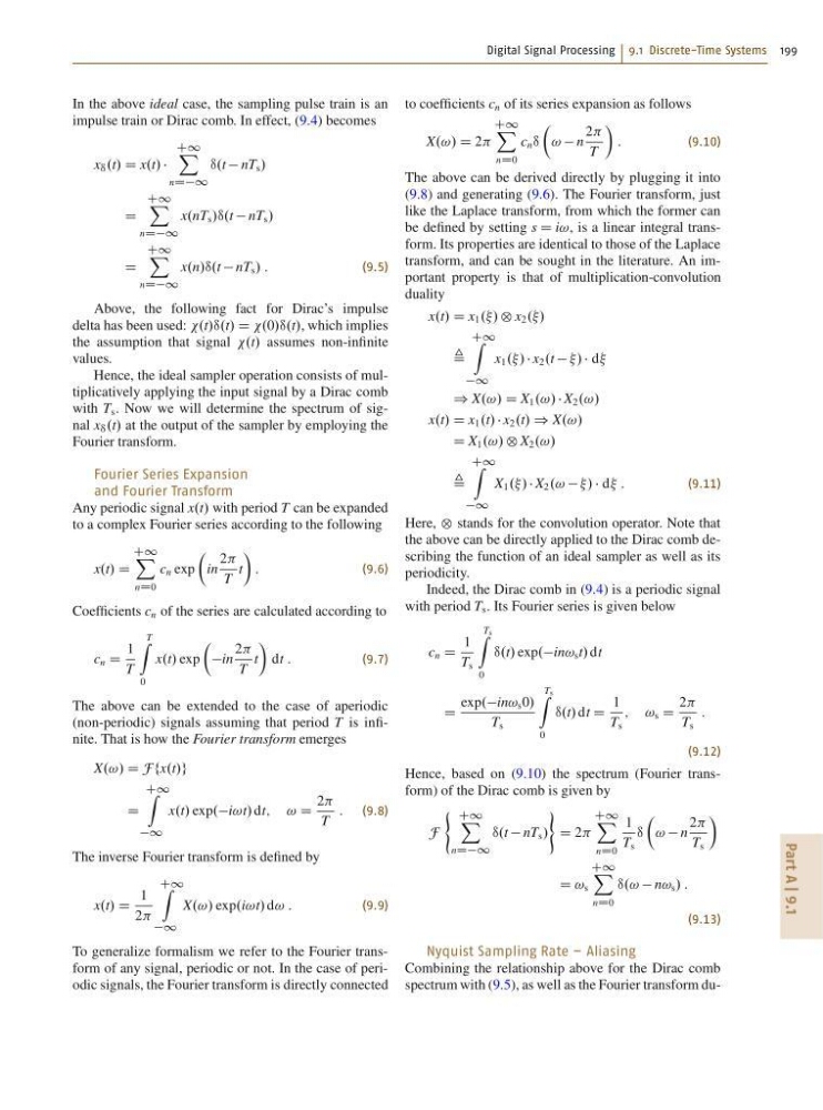
In the above ideal case, the sampling pulse train is an
impulse train or Dirac comb. In effect, (9.4) becomes
x • .t/ D x.t/
C1 X
nDD1
•.t nT s /
D
C1 X
nDD1
x.nT s /•.t nT s /
D
C1 X
nDD1
x.n/•.t nT s / :
(9.5)
Above, the following fact for Dirac’s impulse
delta has been used: .t/•.t/ D .0/•.t/, which implies
the assumption that signal .t/ assumes non-infinite
values.
Hence, the ideal sampler operation consists of multiplicatively applying the input signal by a Dirac comb
with T s . Now we will determine the spectrum of signal x • .t/ at the output of the sampler by employing the
Fourier transform.
Fourier Series Expansion
and Fourier Transform
Any periodic signal x.t/ with period T can be expanded
to a complex Fourier series according to the following
x.t/ D
C1 X
nD0
c n exp
Â
in
2
T
t
Ã
:
(9.6)
Coefficients c n of the series are calculated according to
c n D
1
T
T
Z
0
x.t/ exp
Â
in
2
T
t
Ã
dt :
(9.7)
The above can be extended to the case of aperiodic
(non-periodic) signals assuming that period T is infinite. That is how the Fourier transform emerges
X.!/ D F fx.t/g
D
C1 Z
1
x.t/ exp.i!t/ dt; ! D
2
T
: (9.8)
The inverse Fourier transform is defined by
x.t/ D
1
2
C1 Z
1
X.!/ exp.i!t/ d! :
(9.9)
To generalize formalism we refer to the Fourier transform of any signal, periodic or not. In the case of periodic signals, the Fourier transform is directly connected
to coefficients c n of its series expansion as follows
X.!/ D 2
C1 X
nD0
c n •
Â
! n
2
T
Ã
:
(9.10)
The above can be derived directly by plugging it into
(9.8) and generating (9.6). The Fourier transform, just
like the Laplace transform, from which the former can
be defined by setting s D i!, is a linear integral transform. Its properties are identical to those of the Laplace
transform, and can be sought in the literature. An important property is that of multiplication-convolution
duality
x.t/ D x 1 ../ ˝ x 2 ../
,
C1 Z
1
x 1 ../ x 2 .t / d
) X.!/ D X 1 .!/ X 2 .!/
x.t/ D x 1 .t/ x 2 .t/ ) X.!/
D X 1 .!/ ˝ X 2 .!/
,
C1 Z
1
X 1 ../ X 2 .! / d :
(9.11)
Here, ˝ stands for the convolution operator. Note that
the above can be directly applied to the Dirac comb describing the function of an ideal sampler as well as its
periodicity.
Indeed, the Dirac comb in (9.4) is a periodic signal
with period T s . Its Fourier series is given below
c n D
1
T s
Ts
Z
0
•.t/ exp.in! s t/ dt
D
exp.in! s 0/
T s
Ts
Z
0
•.t/ dt D
1
T s
; ! s D
2
T s
:
(9.12)
Hence, based on (9.10) the spectrum (Fourier transform) of the Dirac comb is given by
F
( C1 X
nDD1
•.t nT s /
)
D 2
C1 X
nD0
1
T s
•
Â
! n
2
T s
Ã
D ! s
C1 X
nD0
•.! n! s / :
(9.13)
Nyquist Sampling Rate – Aliasing
Combining the relationship above for the Dirac comb
spectrum with (9.5), as well as the Fourier transform du-
Part A | 9.1
In the above ideal case, the sampling pulse train is an
impulse train or Dirac comb. In effect, (9.4) becomes
x • .t/ D x.t/
C1 X
nDD1
•.t nT s /
D
C1 X
nDD1
x.nT s /•.t nT s /
D
C1 X
nDD1
x.n/•.t nT s / :
(9.5)
Above, the following fact for Dirac’s impulse
delta has been used: .t/•.t/ D .0/•.t/, which implies
the assumption that signal .t/ assumes non-infinite
values.
Hence, the ideal sampler operation consists of multiplicatively applying the input signal by a Dirac comb
with T s . Now we will determine the spectrum of signal x • .t/ at the output of the sampler by employing the
Fourier transform.
Fourier Series Expansion
and Fourier Transform
Any periodic signal x.t/ with period T can be expanded
to a complex Fourier series according to the following
x.t/ D
C1 X
nD0
c n exp
Â
in
2
T
t
Ã
:
(9.6)
Coefficients c n of the series are calculated according to
c n D
1
T
T
Z
0
x.t/ exp
Â
in
2
T
t
Ã
dt :
(9.7)
The above can be extended to the case of aperiodic
(non-periodic) signals assuming that period T is infinite. That is how the Fourier transform emerges
X.!/ D F fx.t/g
D
C1 Z
1
x.t/ exp.i!t/ dt; ! D
2
T
: (9.8)
The inverse Fourier transform is defined by
x.t/ D
1
2
C1 Z
1
X.!/ exp.i!t/ d! :
(9.9)
To generalize formalism we refer to the Fourier transform of any signal, periodic or not. In the case of periodic signals, the Fourier transform is directly connected
to coefficients c n of its series expansion as follows
X.!/ D 2
C1 X
nD0
c n •
Â
! n
2
T
Ã
:
(9.10)
The above can be derived directly by plugging it into
(9.8) and generating (9.6). The Fourier transform, just
like the Laplace transform, from which the former can
be defined by setting s D i!, is a linear integral transform. Its properties are identical to those of the Laplace
transform, and can be sought in the literature. An important property is that of multiplication-convolution
duality
x.t/ D x 1 ../ ˝ x 2 ../
,
C1 Z
1
x 1 ../ x 2 .t / d
) X.!/ D X 1 .!/ X 2 .!/
x.t/ D x 1 .t/ x 2 .t/ ) X.!/
D X 1 .!/ ˝ X 2 .!/
,
C1 Z
1
X 1 ../ X 2 .! / d :
(9.11)
Here, ˝ stands for the convolution operator. Note that
the above can be directly applied to the Dirac comb describing the function of an ideal sampler as well as its
periodicity.
Indeed, the Dirac comb in (9.4) is a periodic signal
with period T s . Its Fourier series is given below
c n D
1
T s
Ts
Z
0
•.t/ exp.in! s t/ dt
D
exp.in! s 0/
T s
Ts
Z
0
•.t/ dt D
1
T s
; ! s D
2
T s
:
(9.12)
Hence, based on (9.10) the spectrum (Fourier transform) of the Dirac comb is given by
F
( C1 X
nDD1
•.t nT s /
)
D 2
C1 X
nD0
1
T s
•
Â
! n
2
T s
Ã
D ! s
C1 X
nD0
•.! n! s / :
(9.13)
Nyquist Sampling Rate – Aliasing
Combining the relationship above for the Dirac comb
spectrum with (9.5), as well as the Fourier transform du-