

Part A | 9.1
198 Part A Fundamentals
time, computer hardware [9.1, 2]. Since the computer
hardware employed is digital, the signals that can be
processed or generated cannot be continuous time, i. e.,
defined for any instant in time. Instead, the computer
processes and generates tables (i. e., vectors) of values
for the input and output signal, respectively. Such tables
hold the values of the corresponding signals at discrete
time instants and are referred to as discrete-time signals. The time instants for which a discrete-time signal
is known or defined are in most practical cases equally
spaced; this scheme is known as uniform sampling and
the spacing interval between two successive samples of
the signal is mentioned as sampling interval or period.
The systems, e.g., real-time digital hardware, processing discrete-time signals are known as discrete-time
systems. The main advantages in using computers in
marine vehicle or process instrumentation, telecommunications, acoustics etc., instead of analog (continuoustime) systems are [9.1, 3–5]:
1. (Re)use of general purpose hardware for implementing a wide variety of algorithms instead of
custom-built, proprietary designs that may become
obsolete causing higher acquisition and development cost.
2. Changes in the algorithm can be easily implemented
as changes in the software through reprogramming
without need to modify the hardware.
3. Easy implementation of adaptive or time-varying algorithms due to programming.
4. Very small to zero sensitivity to environmental conditions, e.g., ambient temperature, in contrast to,
e.g., analog electric circuitry.
5. Given, well-defined accuracy in computation determined by the computer’s word length.
6. User-friendly human–machine interface (HMI).
7. Network connectivity.
However, there are some disadvantages in using
discrete-time systems, the most important of which is
the need for converter or adapter circuits or interface
systems at their input and output in order to be able to
interact with the vast majority of the real-world physical or engineering systems or processes, which are most
often continuous-time. Such interfaces are the analogto-digital (A/D) and digital-to-analog (D/A) converters.
9.1.2 Signal Sampling
Modeling of Ideal Sampler
Consider a continuous-time signal x.t/, which is driven
through a sampling circuit (sampler) operating at a constant sampling rate (frequency), f s D 1=T s , as shown in
Fig. 9.1.
T s
x (t)
x (n)
Fig. 9.1 Analog signal sampler
The sampler’s output is a sequence of entries of the
sampled signal, x.nT s /, where n is an integer and T s the
sampling period. Sequence x.n/ D x.nT s / is a discretetime signal.
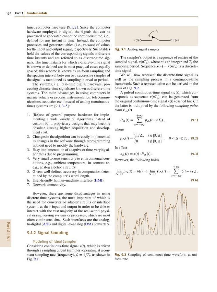
We will now represent the discrete-time signal as
well as the sampling process in a continuous-time
framework. Such a representation can be derived on the
basis of Fig. 9.2.
A pulsed continuous-time signal x .t/, which corresponds to sequence x.nT s /, can be generated from
the original continuous-time signal x.t/ (dashed line), if
the latter is multiplied by the following sampling pulse
train P .t/
P .t/ D
C1 X
nDD1
p .t nT s / ;
(9.1)
where
p .t/ D
(
1=; t 2 Œ0;
0
t … Œ0;
; 0 < T s : (9.2)
In effect
x .t/ D x.t/ P .t/ :
(9.3)
However, the following holds
lim
!0
p .t/ D •.t/ ) lim
!0
P .t/ D
C1 X
nDD1
•.t nT s / :
(9.4)
Fig. 9.2 Sampling of continuous-time waveform at uniform rate
198 Part A Fundamentals
time, computer hardware [9.1, 2]. Since the computer
hardware employed is digital, the signals that can be
processed or generated cannot be continuous time, i. e.,
defined for any instant in time. Instead, the computer
processes and generates tables (i. e., vectors) of values
for the input and output signal, respectively. Such tables
hold the values of the corresponding signals at discrete
time instants and are referred to as discrete-time signals. The time instants for which a discrete-time signal
is known or defined are in most practical cases equally
spaced; this scheme is known as uniform sampling and
the spacing interval between two successive samples of
the signal is mentioned as sampling interval or period.
The systems, e.g., real-time digital hardware, processing discrete-time signals are known as discrete-time
systems. The main advantages in using computers in
marine vehicle or process instrumentation, telecommunications, acoustics etc., instead of analog (continuoustime) systems are [9.1, 3–5]:
1. (Re)use of general purpose hardware for implementing a wide variety of algorithms instead of
custom-built, proprietary designs that may become
obsolete causing higher acquisition and development cost.
2. Changes in the algorithm can be easily implemented
as changes in the software through reprogramming
without need to modify the hardware.
3. Easy implementation of adaptive or time-varying algorithms due to programming.
4. Very small to zero sensitivity to environmental conditions, e.g., ambient temperature, in contrast to,
e.g., analog electric circuitry.
5. Given, well-defined accuracy in computation determined by the computer’s word length.
6. User-friendly human–machine interface (HMI).
7. Network connectivity.
However, there are some disadvantages in using
discrete-time systems, the most important of which is
the need for converter or adapter circuits or interface
systems at their input and output in order to be able to
interact with the vast majority of the real-world physical or engineering systems or processes, which are most
often continuous-time. Such interfaces are the analogto-digital (A/D) and digital-to-analog (D/A) converters.
9.1.2 Signal Sampling
Modeling of Ideal Sampler
Consider a continuous-time signal x.t/, which is driven
through a sampling circuit (sampler) operating at a constant sampling rate (frequency), f s D 1=T s , as shown in
Fig. 9.1.
T s
x (t)
x (n)
Fig. 9.1 Analog signal sampler
The sampler’s output is a sequence of entries of the
sampled signal, x.nT s /, where n is an integer and T s the
sampling period. Sequence x.n/ D x.nT s / is a discretetime signal.
We will now represent the discrete-time signal as
well as the sampling process in a continuous-time
framework. Such a representation can be derived on the
basis of Fig. 9.2.
A pulsed continuous-time signal x .t/, which corresponds to sequence x.nT s /, can be generated from
the original continuous-time signal x.t/ (dashed line), if
the latter is multiplied by the following sampling pulse
train P .t/
P .t/ D
C1 X
nDD1
p .t nT s / ;
(9.1)
where
p .t/ D
(
1=; t 2 Œ0;
0
t … Œ0;
; 0 < T s : (9.2)
In effect
x .t/ D x.t/ P .t/ :
(9.3)
However, the following holds
lim
!0
p .t/ D •.t/ ) lim
!0
P .t/ D
C1 X
nDD1
•.t nT s / :
(9.4)
Fig. 9.2 Sampling of continuous-time waveform at uniform rate