

Ocean Electromagnetics 8.6 Magnetic and Electric Dipoles in an Unbounded Ocean 187
Part A | 8.6
where r is the radial distance from the origin as shown
in Fig. 8.8. Converting (8.98) to spherical coordinates
and placing it into (8.92) and (8.93), the electric and
magnetic fields of a point electric dipole in an unbounded ocean are written as
E r D
p cos Â
2r 3 .1 C r/e
r
;
(8.99)
E ™ D
p sin Â
4r 3 .1 C r C
2 r
2
/e
r
;
(8.100)
H ® D
p sin Â
4r 2 .1 C r/e
r
:
(8.101)
If the point dipole was located at coordinates .x 0 ; y 0 ; z 0 /
instead of the origin, then r becomes
p
.x x 0 / 2 C .y y 0 / 2 C .z z 0 / 2 :
The derivation of a magnetic point dipole follows
that shown above for the electric. In this case, the magnetic point dipole has a source strength m that is also
located at the origin, and is aligned along the z-axis.
A dipole of this type could be produced by an electric current flowing in the ' direction of the coordinate
system in Fig. 8.8. This is mathematically equivalent
to a virtual magnetic current source aligned along the
z-axis. Therefore, the equivalent impressed magnetic
current density for this dipole can be written as
M i D O
a z m•.x
0
/•.y
0
/•.z
0
/ :
(8.102)
Using (8.102) in (8.95) yields the electric vector potential
F z D
"me
r
4r
:
(8.103)
Converting (8.103) to spherical coordinates and placing
it into (8.92) and (8.93), the electric and magnetic fields
of a point magnetic dipole in an unbounded ocean can
be written as
H r D
m cos Â
2r 3 .1 C r/e
r
;
(8.104)
H ™ D
m sin Â
4r 3 .1 C r C
2 r
2
/e
r
;
(8.105)
E ® D
i!!m sin Â
4r 2
.1 C r/e
r
:
(8.106)
It should be noted that the electromagnetic fields for
both the electric and magnetic dipole sources are circularly symmetric and are not a function of the '
coordinate.
The equations for the electromagnetic fields of electric and magnetic point dipoles in an unbounded ocean
reduce to the standard static magnetic and electric expressions by setting the frequency in (8.99) to (8.101)
and (8.104) to (8.106) to zero. Carrying this out gives
the electric and magnetic fields of a static electric dipole
in an unbounded ocean as
E r D
p cos Â
2r 3 ;
(8.107)
E ™ D
p sin Â
4r 3 ;
(8.108)
H ® D
p sin Â
4r 2 ;
(8.109)
and for the static magnetic dipole (8.104) to (8.106) reduce to
H r D
m cos Â
2r 3 ;
(8.110)
H ™ D
m sin Â
4r 3 ;
(8.111)
E ® D 0 :
(8.112)
It should be noted that all electric and magnetic field
components for static dipoles fall off in the radial direction as r
3 except for the ' component of the magnetic
field of the static electric dipole, which fall off as r
2 ,
and the ' component of the electric field of the static
magnetic dipole, which is zero.
Except for the zero E ® component of the static
magnetic dipole, the static and time-harmonic dipole
equations differ by a factor of either .1 C r/e
”r or
.1 C r C
2 r
2
/e
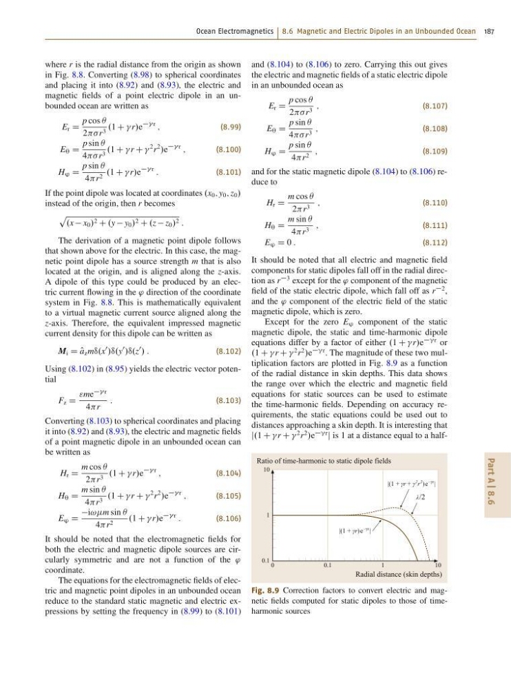
”r . The magnitude of these two multiplication factors are plotted in Fig. 8.9 as a function
of the radial distance in skin depths. This data shows
the range over which the electric and magnetic field
equations for static sources can be used to estimate
the time-harmonic fields. Depending on accuracy requirements, the static equations could be used out to
distances approaching a skin depth. It is interesting that
j.1 C r C
2 r
2
/e
”r
j is 1 at a distance equal to a half0
0.1
1
|(1 + γr)e
–γr |
|(1 + γr + γ
2 r
2 )e
–γr |
λ/2
10
Radial distance (skin depths)
Ratio of time-harmonic to static dipole fields
10
1
0.1
Fig. 8.9 Correction factors to convert electric and magnetic fields computed for static dipoles to those of timeharmonic sources
Part A | 8.6
where r is the radial distance from the origin as shown
in Fig. 8.8. Converting (8.98) to spherical coordinates
and placing it into (8.92) and (8.93), the electric and
magnetic fields of a point electric dipole in an unbounded ocean are written as
E r D
p cos Â
2r 3 .1 C r/e
r
;
(8.99)
E ™ D
p sin Â
4r 3 .1 C r C
2 r
2
/e
r
;
(8.100)
H ® D
p sin Â
4r 2 .1 C r/e
r
:
(8.101)
If the point dipole was located at coordinates .x 0 ; y 0 ; z 0 /
instead of the origin, then r becomes
p
.x x 0 / 2 C .y y 0 / 2 C .z z 0 / 2 :
The derivation of a magnetic point dipole follows
that shown above for the electric. In this case, the magnetic point dipole has a source strength m that is also
located at the origin, and is aligned along the z-axis.
A dipole of this type could be produced by an electric current flowing in the ' direction of the coordinate
system in Fig. 8.8. This is mathematically equivalent
to a virtual magnetic current source aligned along the
z-axis. Therefore, the equivalent impressed magnetic
current density for this dipole can be written as
M i D O
a z m•.x
0
/•.y
0
/•.z
0
/ :
(8.102)
Using (8.102) in (8.95) yields the electric vector potential
F z D
"me
r
4r
:
(8.103)
Converting (8.103) to spherical coordinates and placing
it into (8.92) and (8.93), the electric and magnetic fields
of a point magnetic dipole in an unbounded ocean can
be written as
H r D
m cos Â
2r 3 .1 C r/e
r
;
(8.104)
H ™ D
m sin Â
4r 3 .1 C r C
2 r
2
/e
r
;
(8.105)
E ® D
i!!m sin Â
4r 2
.1 C r/e
r
:
(8.106)
It should be noted that the electromagnetic fields for
both the electric and magnetic dipole sources are circularly symmetric and are not a function of the '
coordinate.
The equations for the electromagnetic fields of electric and magnetic point dipoles in an unbounded ocean
reduce to the standard static magnetic and electric expressions by setting the frequency in (8.99) to (8.101)
and (8.104) to (8.106) to zero. Carrying this out gives
the electric and magnetic fields of a static electric dipole
in an unbounded ocean as
E r D
p cos Â
2r 3 ;
(8.107)
E ™ D
p sin Â
4r 3 ;
(8.108)
H ® D
p sin Â
4r 2 ;
(8.109)
and for the static magnetic dipole (8.104) to (8.106) reduce to
H r D
m cos Â
2r 3 ;
(8.110)
H ™ D
m sin Â
4r 3 ;
(8.111)
E ® D 0 :
(8.112)
It should be noted that all electric and magnetic field
components for static dipoles fall off in the radial direction as r
3 except for the ' component of the magnetic
field of the static electric dipole, which fall off as r
2 ,
and the ' component of the electric field of the static
magnetic dipole, which is zero.
Except for the zero E ® component of the static
magnetic dipole, the static and time-harmonic dipole
equations differ by a factor of either .1 C r/e
”r or
.1 C r C
2 r
2
/e
”r . The magnitude of these two multiplication factors are plotted in Fig. 8.9 as a function
of the radial distance in skin depths. This data shows
the range over which the electric and magnetic field
equations for static sources can be used to estimate
the time-harmonic fields. Depending on accuracy requirements, the static equations could be used out to
distances approaching a skin depth. It is interesting that
j.1 C r C
2 r
2
/e
”r
j is 1 at a distance equal to a half0
0.1
1
|(1 + γr)e
–γr |
|(1 + γr + γ
2 r
2 )e
–γr |
λ/2
10
Radial distance (skin depths)
Ratio of time-harmonic to static dipole fields
10
1
0.1
Fig. 8.9 Correction factors to convert electric and magnetic fields computed for static dipoles to those of timeharmonic sources