

Part A | 7.3
172 Part A Fundamentals
far-field axial velocity in the jet at a distance x downstream of the hole can be shown to be given by
u D
3J
8x
Â
1 C
3JÁ
2
64 2
à 2
:
(7.83)
Thus the speed decreases approximately linearly with
downstream distance.
Finally, velocity associated with a two-dimensional
laminar shear layer where the streamwise speed u
transitions from U 2 to U across the layer may be represented by Blasius type profiles [7.37] upon introducing
the similarity variable Á D y
p
U=.2x/ as u D UF
0
.Á/,
and v D
p
U=.2x/.ÁF
0
F/, where F.Á/ satisfies
F
000
C FF
00
D 0 ; F.0/ D 0 ;
F
0
.1/ D
U
U 2
; F
0
.1/ D 1 :
(7.84)
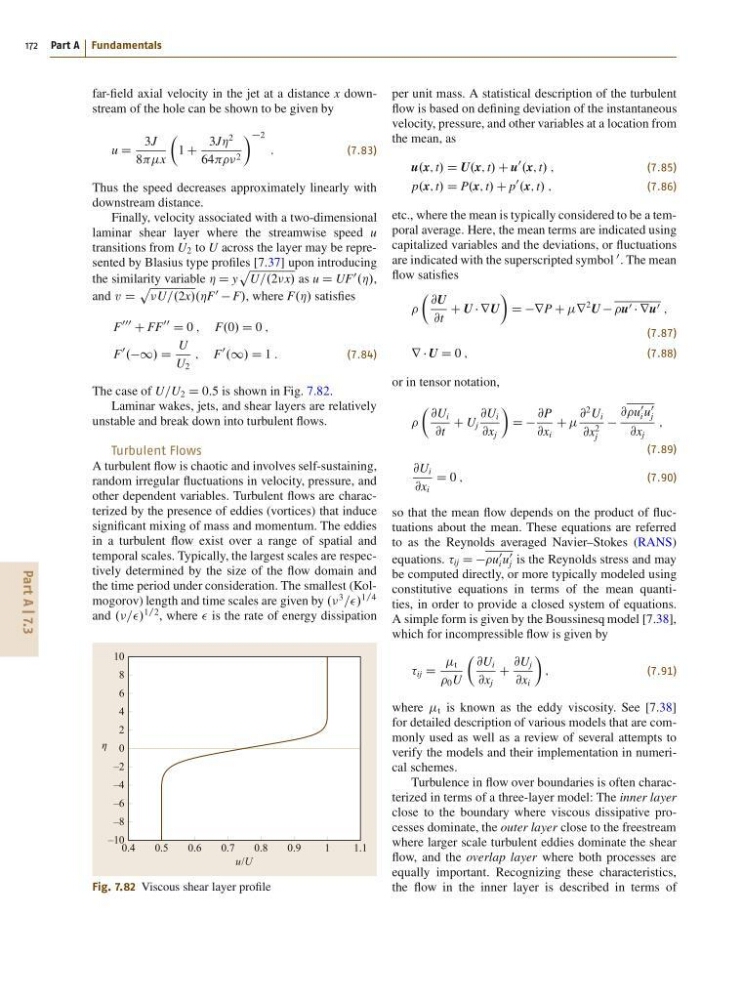
The case of U=U 2 D 0:5 is shown in Fig. 7.82.
Laminar wakes, jets, and shear layers are relatively
unstable and break down into turbulent flows.
Turbulent Flows
A turbulent flow is chaotic and involves self-sustaining,
random irregular fluctuations in velocity, pressure, and
other dependent variables. Turbulent flows are characterized by the presence of eddies (vortices) that induce
significant mixing of mass and momentum. The eddies
in a turbulent flow exist over a range of spatial and
temporal scales. Typically, the largest scales are respectively determined by the size of the flow domain and
the time period under consideration. The smallest (Kolmogorov) length and time scales are given by ..
3
==/
1=4
and ..==/
1=2 , where is the rate of energy dissipation
0.4
0.5
0.6
0.7
0.8
0.9
1
1.1
η
u/U
10
8
6
4
2
0
–2
–4
–6
–8
–10
Fig. 7.82 Viscous shear layer profile
per unit mass. A statistical description of the turbulent
flow is based on defining deviation of the instantaneous
velocity, pressure, and other variables at a location from
the mean, as
u.x; t/ D U.x; t/ C u
0
.x; t/ ;
(7.85)
p.x; t/ D P.x; t/ C p
0
.x; t/ ;
(7.86)
etc., where the mean is typically considered to be a temporal average. Here, the mean terms are indicated using
capitalized variables and the deviations, or fluctuations
are indicated with the superscripted symbol
0 . The mean
flow satisfies
 @U
@t
C U rU
Ã
D DrP C r
2 U u 0 ru 0 ;
(7.87)
r r U D 0 ;
(7.88)
or in tensor notation,
 @U i
@t
C U j
@U i
@x j
Ã
D D
@P
@x i
C
@
2 U i
@x
2
j
@u
0
i u
0
j
@x j
;
(7.89)
@U i
@x i
D 0 ;
(7.90)
so that the mean flow depends on the product of fluctuations about the mean. These equations are referred
to as the Reynolds averaged Navier–Stokes (RANS)
equations. ij D Du
0
i u
0
j is the Reynolds stress and may
be computed directly, or more typically modeled using
constitutive equations in terms of the mean quantities, in order to provide a closed system of equations.
A simple form is given by the Boussinesq model [7.38],
which for incompressible flow is given by
ij D
t
0 U
 @U i
@x j
C
@U j
@x i
Ã
;
(7.91)
where t is known as the eddy viscosity. See [7.38]
for detailed description of various models that are commonly used as well as a review of several attempts to
verify the models and their implementation in numerical schemes.
Turbulence in flow over boundaries is often characterized in terms of a three-layer model: The inner layer
close to the boundary where viscous dissipative processes dominate, the outer layer close to the freestream
where larger scale turbulent eddies dominate the shear
flow, and the overlap layer where both processes are
equally important. Recognizing these characteristics,
the flow in the inner layer is described in terms of
172 Part A Fundamentals
far-field axial velocity in the jet at a distance x downstream of the hole can be shown to be given by
u D
3J
8x
Â
1 C
3JÁ
2
64 2
à 2
:
(7.83)
Thus the speed decreases approximately linearly with
downstream distance.
Finally, velocity associated with a two-dimensional
laminar shear layer where the streamwise speed u
transitions from U 2 to U across the layer may be represented by Blasius type profiles [7.37] upon introducing
the similarity variable Á D y
p
U=.2x/ as u D UF
0
.Á/,
and v D
p
U=.2x/.ÁF
0
F/, where F.Á/ satisfies
F
000
C FF
00
D 0 ; F.0/ D 0 ;
F
0
.1/ D
U
U 2
; F
0
.1/ D 1 :
(7.84)
The case of U=U 2 D 0:5 is shown in Fig. 7.82.
Laminar wakes, jets, and shear layers are relatively
unstable and break down into turbulent flows.
Turbulent Flows
A turbulent flow is chaotic and involves self-sustaining,
random irregular fluctuations in velocity, pressure, and
other dependent variables. Turbulent flows are characterized by the presence of eddies (vortices) that induce
significant mixing of mass and momentum. The eddies
in a turbulent flow exist over a range of spatial and
temporal scales. Typically, the largest scales are respectively determined by the size of the flow domain and
the time period under consideration. The smallest (Kolmogorov) length and time scales are given by ..
3
==/
1=4
and ..==/
1=2 , where is the rate of energy dissipation
0.4
0.5
0.6
0.7
0.8
0.9
1
1.1
η
u/U
10
8
6
4
2
0
–2
–4
–6
–8
–10
Fig. 7.82 Viscous shear layer profile
per unit mass. A statistical description of the turbulent
flow is based on defining deviation of the instantaneous
velocity, pressure, and other variables at a location from
the mean, as
u.x; t/ D U.x; t/ C u
0
.x; t/ ;
(7.85)
p.x; t/ D P.x; t/ C p
0
.x; t/ ;
(7.86)
etc., where the mean is typically considered to be a temporal average. Here, the mean terms are indicated using
capitalized variables and the deviations, or fluctuations
are indicated with the superscripted symbol
0 . The mean
flow satisfies
 @U
@t
C U rU
Ã
D DrP C r
2 U u 0 ru 0 ;
(7.87)
r r U D 0 ;
(7.88)
or in tensor notation,
 @U i
@t
C U j
@U i
@x j
Ã
D D
@P
@x i
C
@
2 U i
@x
2
j
@u
0
i u
0
j
@x j
;
(7.89)
@U i
@x i
D 0 ;
(7.90)
so that the mean flow depends on the product of fluctuations about the mean. These equations are referred
to as the Reynolds averaged Navier–Stokes (RANS)
equations. ij D Du
0
i u
0
j is the Reynolds stress and may
be computed directly, or more typically modeled using
constitutive equations in terms of the mean quantities, in order to provide a closed system of equations.
A simple form is given by the Boussinesq model [7.38],
which for incompressible flow is given by
ij D
t
0 U
 @U i
@x j
C
@U j
@x i
Ã
;
(7.91)
where t is known as the eddy viscosity. See [7.38]
for detailed description of various models that are commonly used as well as a review of several attempts to
verify the models and their implementation in numerical schemes.
Turbulence in flow over boundaries is often characterized in terms of a three-layer model: The inner layer
close to the boundary where viscous dissipative processes dominate, the outer layer close to the freestream
where larger scale turbulent eddies dominate the shear
flow, and the overlap layer where both processes are
equally important. Recognizing these characteristics,
the flow in the inner layer is described in terms of