

Hydromechanics 7.3 Hydrodynamics 169
Part A | 7.3
Therefore,
D k ln r m D 1 C 2 D
7
4 ln.10/
ln r  :
Then, we have the system
1 D k ln r D n! ;
2 D DÂ D n! :
Solving the system for r gives
r D e
Â=k
D e
n!=k
D expŒln 10
n=7
D 10
n=7
:
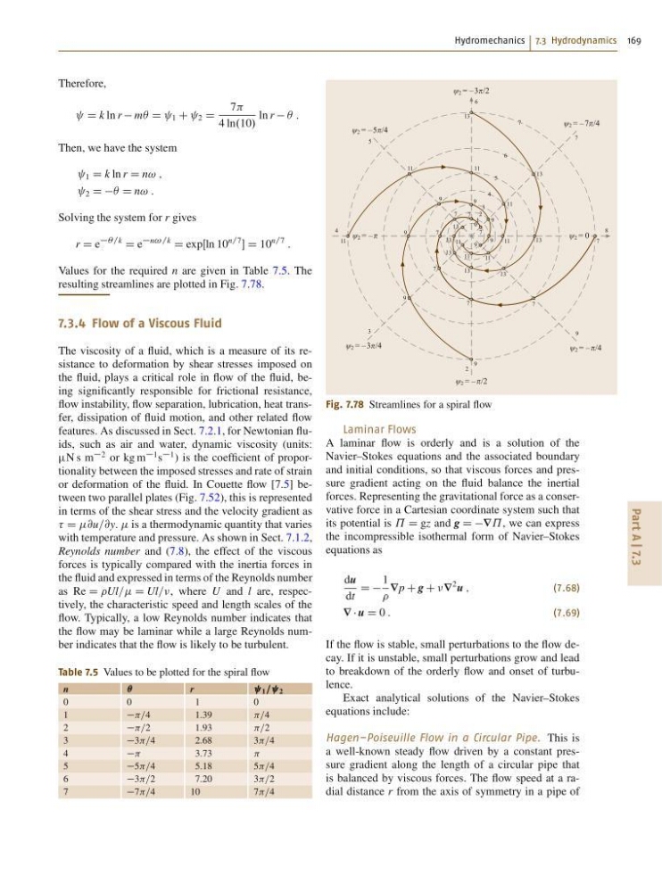
Values for the required n are given in Table 7.5. The
resulting streamlines are plotted in Fig. 7.78.
7.3.4 Flow of a Viscous Fluid
The viscosity of a fluid, which is a measure of its resistance to deformation by shear stresses imposed on
the fluid, plays a critical role in flow of the fluid, being significantly responsible for frictional resistance,
flow instability, flow separation, lubrication, heat transfer, dissipation of fluid motion, and other related flow
features. As discussed in Sect. 7.2.1, for Newtonian fluids, such as air and water, dynamic viscosity (units:
N s m
2 or kg m
1 s
1 ) is the coefficient of proportionality between the imposed stresses and rate of strain
or deformation of the fluid. In Couette flow [7.5] between two parallel plates (Fig. 7.52), this is represented
in terms of the shear stress and the velocity gradient as
D @u=@y. is a thermodynamic quantity that varies
with temperature and pressure. As shown in Sect. 7.1.2,
Reynolds number and (7.8), the effect of the viscous
forces is typically compared with the inertia forces in
the fluid and expressed in terms of the Reynolds number
as Re D Ul== D Ul==, where U and l are, respectively, the characteristic speed and length scales of the
flow. Typically, a low Reynolds number indicates that
the flow may be laminar while a large Reynolds number indicates that the flow is likely to be turbulent.
Table 7.5 Values to be plotted for the spiral flow
n
Â
r
1 = 2
0
0
1
0
1
=4
1:39
=4
2
=2
1:93
=2
3
3=4
2:68
3=4
4
3:73
5
5=4
5:18
5=4
6
3=2
7:20
3=2
7
7=4
10
7=4
ψ 2 = – 3/4
ψ 2 = – 3/2
ψ 2 = – 7/4
ψ 2 = – 5/4
ψ 2 = – /2
ψ 2 = – /4
ψ 2 = 0
ψ 2 = –
3
9
9
2
9
9
9
9
9
9
0
1
2
3
4
4
5
5
6
6
7
11
11
11
11
11
11
11
11
13
13
13
13
13
13
7
8
9
7
7
7
7
7
7
7
7
13
13
Fig. 7.78 Streamlines for a spiral flow
Laminar Flows
A laminar flow is orderly and is a solution of the
Navier–Stokes equations and the associated boundary
and initial conditions, so that viscous forces and pressure gradient acting on the fluid balance the inertial
forces. Representing the gravitational force as a conservative force in a Cartesian coordinate system such that
its potential is ˘ D gz and g D Dr ˘ , we can express
the incompressible isothermal form of Navier–Stokes
equations as
du
dt
D D
1
r p C g C r
2 u ;
(7.68)
r u D 0 :
(7.69)
If the flow is stable, small perturbations to the flow decay. If it is unstable, small perturbations grow and lead
to breakdown of the orderly flow and onset of turbulence.
Exact analytical solutions of the Navier–Stokes
equations include:
Hagen–Poiseuille Flow in a Circular Pipe. This is
a well-known steady flow driven by a constant pressure gradient along the length of a circular pipe that
is balanced by viscous forces. The flow speed at a radial distance r from the axis of symmetry in a pipe of
Part A | 7.3
Therefore,
D k ln r m D 1 C 2 D
7
4 ln.10/
ln r  :
Then, we have the system
1 D k ln r D n! ;
2 D DÂ D n! :
Solving the system for r gives
r D e
Â=k
D e
n!=k
D expŒln 10
n=7
D 10
n=7
:
Values for the required n are given in Table 7.5. The
resulting streamlines are plotted in Fig. 7.78.
7.3.4 Flow of a Viscous Fluid
The viscosity of a fluid, which is a measure of its resistance to deformation by shear stresses imposed on
the fluid, plays a critical role in flow of the fluid, being significantly responsible for frictional resistance,
flow instability, flow separation, lubrication, heat transfer, dissipation of fluid motion, and other related flow
features. As discussed in Sect. 7.2.1, for Newtonian fluids, such as air and water, dynamic viscosity (units:
N s m
2 or kg m
1 s
1 ) is the coefficient of proportionality between the imposed stresses and rate of strain
or deformation of the fluid. In Couette flow [7.5] between two parallel plates (Fig. 7.52), this is represented
in terms of the shear stress and the velocity gradient as
D @u=@y. is a thermodynamic quantity that varies
with temperature and pressure. As shown in Sect. 7.1.2,
Reynolds number and (7.8), the effect of the viscous
forces is typically compared with the inertia forces in
the fluid and expressed in terms of the Reynolds number
as Re D Ul== D Ul==, where U and l are, respectively, the characteristic speed and length scales of the
flow. Typically, a low Reynolds number indicates that
the flow may be laminar while a large Reynolds number indicates that the flow is likely to be turbulent.
Table 7.5 Values to be plotted for the spiral flow
n
Â
r
1 = 2
0
0
1
0
1
=4
1:39
=4
2
=2
1:93
=2
3
3=4
2:68
3=4
4
3:73
5
5=4
5:18
5=4
6
3=2
7:20
3=2
7
7=4
10
7=4
ψ 2 = – 3/4
ψ 2 = – 3/2
ψ 2 = – 7/4
ψ 2 = – 5/4
ψ 2 = – /2
ψ 2 = – /4
ψ 2 = 0
ψ 2 = –
3
9
9
2
9
9
9
9
9
9
0
1
2
3
4
4
5
5
6
6
7
11
11
11
11
11
11
11
11
13
13
13
13
13
13
7
8
9
7
7
7
7
7
7
7
7
13
13
Fig. 7.78 Streamlines for a spiral flow
Laminar Flows
A laminar flow is orderly and is a solution of the
Navier–Stokes equations and the associated boundary
and initial conditions, so that viscous forces and pressure gradient acting on the fluid balance the inertial
forces. Representing the gravitational force as a conservative force in a Cartesian coordinate system such that
its potential is ˘ D gz and g D Dr ˘ , we can express
the incompressible isothermal form of Navier–Stokes
equations as
du
dt
D D
1
r p C g C r
2 u ;
(7.68)
r u D 0 :
(7.69)
If the flow is stable, small perturbations to the flow decay. If it is unstable, small perturbations grow and lead
to breakdown of the orderly flow and onset of turbulence.
Exact analytical solutions of the Navier–Stokes
equations include:
Hagen–Poiseuille Flow in a Circular Pipe. This is
a well-known steady flow driven by a constant pressure gradient along the length of a circular pipe that
is balanced by viscous forces. The flow speed at a radial distance r from the axis of symmetry in a pipe of