

Part A | 7.3
164 Part A Fundamentals
d) Doublet
Let a ! 0 in the source/sink flow above, we
have
D
m
2
ln
 r 1
r 2
Ã
:
From geometry, r 1 D 2a cos  1 Cr 2 cos. 2  1 /.
Therefore,
D
m
2
ln
 2a cos  1
r 2
C cos. 2  1 /
Ã
:
When a ! 0 but m is increased such that ma==
remains finite and constant, r 2 ! r, Â 2 ! Â , and
cos. 2  1 / ! 1 so that
lim
a!0
D
m
2
ln
 2a cos Â
r
C 1
Ã
:
A Taylor’s series expansion of the argument
about 1 gives
D
ma cos Â
r
D
x
x 2 C y 2 :
Similarly, for small angles tan   and
D D
m
2
Â
2ay
x 2 C y 2
Ã
D D
ma
Â
y
x 2 C y 2
Ã
;
D D
y
x 2 C y 2 :
With r
2
D x
2
C y
2 so that cos  D x=r and
sin  D y=r,
D
cos Â
r
and D D
sin Â
r
:
x
y
Fig. 7.64 Rankine body flow
The complex velocity potential is then
w .z/ D C i D
r
.cos  i sin Â/
D
e
iÂ
r
D
z
:
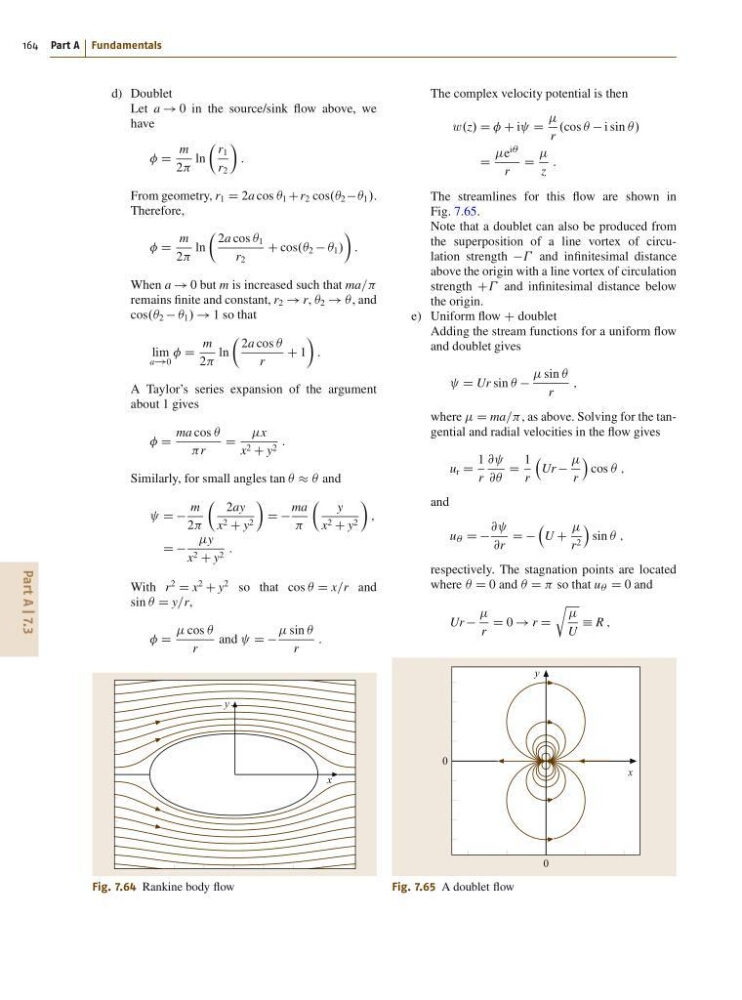
The streamlines for this flow are shown in
Fig. 7.65.
Note that a doublet can also be produced from
the superposition of a line vortex of circulation strength and infinitesimal distance
above the origin with a line vortex of circulation
strength C and infinitesimal distance below
the origin.
e) Uniform flow C doublet
Adding the stream functions for a uniform flow
and doublet gives
D Ur sin Â
sin Â
r
;
where D ma==, as above. Solving for the tangential and radial velocities in the flow gives
u r D
1
r
@
@Â
D
1
r
Ur
r
Á
cos  ;
and
u  D D
@
@r
D D
U C
r 2
Á
sin  ;
respectively. The stagnation points are located
where  D 0 and  D so that u  D 0 and
Ur
r
D 0 ! r D
r
U
Á R ;
x
y
0
0
Fig. 7.65 A doublet flow
164 Part A Fundamentals
d) Doublet
Let a ! 0 in the source/sink flow above, we
have
D
m
2
ln
 r 1
r 2
Ã
:
From geometry, r 1 D 2a cos  1 Cr 2 cos. 2  1 /.
Therefore,
D
m
2
ln
 2a cos  1
r 2
C cos. 2  1 /
Ã
:
When a ! 0 but m is increased such that ma==
remains finite and constant, r 2 ! r, Â 2 ! Â , and
cos. 2  1 / ! 1 so that
lim
a!0
D
m
2
ln
 2a cos Â
r
C 1
Ã
:
A Taylor’s series expansion of the argument
about 1 gives
D
ma cos Â
r
D
x
x 2 C y 2 :
Similarly, for small angles tan   and
D D
m
2
Â
2ay
x 2 C y 2
Ã
D D
ma
Â
y
x 2 C y 2
Ã
;
D D
y
x 2 C y 2 :
With r
2
D x
2
C y
2 so that cos  D x=r and
sin  D y=r,
D
cos Â
r
and D D
sin Â
r
:
x
y
Fig. 7.64 Rankine body flow
The complex velocity potential is then
w .z/ D C i D
r
.cos  i sin Â/
D
e
iÂ
r
D
z
:
The streamlines for this flow are shown in
Fig. 7.65.
Note that a doublet can also be produced from
the superposition of a line vortex of circulation strength and infinitesimal distance
above the origin with a line vortex of circulation
strength C and infinitesimal distance below
the origin.
e) Uniform flow C doublet
Adding the stream functions for a uniform flow
and doublet gives
D Ur sin Â
sin Â
r
;
where D ma==, as above. Solving for the tangential and radial velocities in the flow gives
u r D
1
r
@
@Â
D
1
r
Ur
r
Á
cos  ;
and
u  D D
@
@r
D D
U C
r 2
Á
sin  ;
respectively. The stagnation points are located
where  D 0 and  D so that u  D 0 and
Ur
r
D 0 ! r D
r
U
Á R ;
x
y
0
0
Fig. 7.65 A doublet flow