

Hydromechanics 7.3 Hydrodynamics 163
Part A | 7.3
m
2
ψ stag =
–2 –1.5 –1 –0.5
0
0.5
x
y
1
1.5
2
Stagnation point
2
1.5
1
0.5
0
–0.5
–1
–1.5
–2
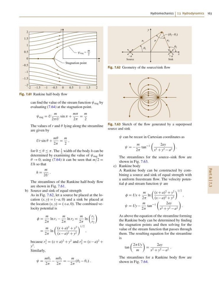
Fig. 7.61 Rankine half-body flow
can find the value of the stream function stag by
evaluating (7.64) at the stagnation point.
stag D U
m
2U
sin C
m
2
D
m
2
The values of r and  lying along the streamline
are given by
Ur sin  C
mÂ
2
D
m
2
;
for 0 Ä Â Ä . The
1
2
width of the body h can be
determined by examining the value of stag for
 ! 0; using (7.64) it can be seen that m=2 D
Uh so that
h D
m
2U
:
The streamlines of the Rankine half-body flow
are shown in Fig. 7.61.
b) Source and sink of equal strength
As in Fig. 7.62, let a source be placed at the location .x; y/ D .a; 0/ and a sink be placed at
the location .x; y/ D .Ca; 0/. The combined velocity potential is
D
m
2
ln r 1
m
2
ln r 2 D
m
2
ln
 r 1
r 2
Ã
D
m
2
ln
 .x C a/
2
C y
2
.x a/ 2 C y 2
à 1=2
;
because r
2
1 D .x C a/
2
C y
2 and r
2
2 D .x a/
2
C
y
2 .
Similarly,
D
m 1
2
m 2
2
D D
m
2
. 2  1 / :
θ 1
θ 2
(θ 2 – θ 1 )
–a
Source
+a
Sink
y
x
r 1
r 2
r
Fig. 7.62 Geometry of the source/sink flow
Fig. 7.63 Sketch of the flow generated by a superposed
source and sink
can be recast in Cartesian coordinates as
D D
m
2
tan
1
Â
2ay
x 2 C y 2 a 2
Ã
:
The streamlines for the source–sink flow are
shown in Fig. 7.63.
c) Rankine body
A Rankine body can be constructed by combining a source and sink of equal strength with
a uniform freestream flow. The velocity potential and stream function are
D Ux C
m
2
ln
 .x C a/
2
C y
2
.x a/ 2 C y 2
à 1=2
;
D Uy
m
2
tan
1
Â
2ay
x 2 C y 2 a 2
Ã
:
As above the equation of the streamline forming
the Rankine body can be determined by finding
the stagnation points and then solving for the
value of the stream function that passes through
them. The resulting equation for the streamline
is
tan
 2Uy
m
Ã
D
2ay
x 2 C y 2 a 2 :
The streamlines for a Rankine body flow are
shown in Fig. 7.64.
Part A | 7.3
m
2
ψ stag =
–2 –1.5 –1 –0.5
0
0.5
x
y
1
1.5
2
Stagnation point
2
1.5
1
0.5
0
–0.5
–1
–1.5
–2
Fig. 7.61 Rankine half-body flow
can find the value of the stream function stag by
evaluating (7.64) at the stagnation point.
stag D U
m
2U
sin C
m
2
D
m
2
The values of r and  lying along the streamline
are given by
Ur sin  C
mÂ
2
D
m
2
;
for 0 Ä Â Ä . The
1
2
width of the body h can be
determined by examining the value of stag for
 ! 0; using (7.64) it can be seen that m=2 D
Uh so that
h D
m
2U
:
The streamlines of the Rankine half-body flow
are shown in Fig. 7.61.
b) Source and sink of equal strength
As in Fig. 7.62, let a source be placed at the location .x; y/ D .a; 0/ and a sink be placed at
the location .x; y/ D .Ca; 0/. The combined velocity potential is
D
m
2
ln r 1
m
2
ln r 2 D
m
2
ln
 r 1
r 2
Ã
D
m
2
ln
 .x C a/
2
C y
2
.x a/ 2 C y 2
à 1=2
;
because r
2
1 D .x C a/
2
C y
2 and r
2
2 D .x a/
2
C
y
2 .
Similarly,
D
m 1
2
m 2
2
D D
m
2
. 2  1 / :
θ 1
θ 2
(θ 2 – θ 1 )
–a
Source
+a
Sink
y
x
r 1
r 2
r
Fig. 7.62 Geometry of the source/sink flow
Fig. 7.63 Sketch of the flow generated by a superposed
source and sink
can be recast in Cartesian coordinates as
D D
m
2
tan
1
Â
2ay
x 2 C y 2 a 2
Ã
:
The streamlines for the source–sink flow are
shown in Fig. 7.63.
c) Rankine body
A Rankine body can be constructed by combining a source and sink of equal strength with
a uniform freestream flow. The velocity potential and stream function are
D Ux C
m
2
ln
 .x C a/
2
C y
2
.x a/ 2 C y 2
à 1=2
;
D Uy
m
2
tan
1
Â
2ay
x 2 C y 2 a 2
Ã
:
As above the equation of the streamline forming
the Rankine body can be determined by finding
the stagnation points and then solving for the
value of the stream function that passes through
them. The resulting equation for the streamline
is
tan
 2Uy
m
Ã
D
2ay
x 2 C y 2 a 2 :
The streamlines for a Rankine body flow are
shown in Fig. 7.64.